ED09: Electrostatic Boundary Value Problems, Conductors, and Image Charges
ED08 calculated electric fields when the source charge was prescribed. In this article, a different
kind of problem is considered: the positions and shapes of conducting boundaries are known, but
the charge distribution over those boundaries is not known in advance. The electric field causes
charges to move until electrostatic equilibrium is reached. The final charge distribution is therefore
part of the answer.
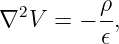
Instead of calculating the field directly from a known charge distribution, we often solve for the
scalar potential V from
with a specification of the potential or its Normal derivative along the boundary. Here 𝜖 is the
constant permittivity of the homogeneous region under consideration. In regions without free
charge,
This is Laplace’s equation. The electrostatic field is recovered from
We will derive Conductor boundary conditions, prove the uniqueness theorem, construct
image-charge solutions for a grounded plane and a grounded sphere, and use separation of variables
to solve a boundary value problem that cannot be reduced to one image charge. The emphasis is
on showing every important step and using the uniqueness theorem to explain why each
construction is valid.
1 What is a boundary value problem?
Consider a region Ω bounded by a surface S = ∂Ω. A typical electrostatic problem consists of
- a differential equation, such as Poisson’s or Laplace’s equation;
- a geometric region in which the equation holds;
- source charges specified within the region, when present;
- and data on the boundary that select a physical solution.
There are two especially important kinds of boundary data.
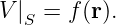
1.1 Specified potential: the Dirichlet condition
On the boundary,
For example, a grounded conductor has V = 0 relative to the chosen ground reference. A conductor
held by a voltage source at fixed potential V 0 has V = V 0 on its surface.
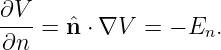
1.2 Specified normal derivative: the Neumann condition
Let n point outward from Ω. If the normal electric field is specified, then
Thus a Neumann boundary condition specifies ∂V∕∂n, rather than V itself. A boundary condition
specifying one of these quantities should not be confused with one specifying the conductor’s total
charge. They are related, but not generally the same kind of data.
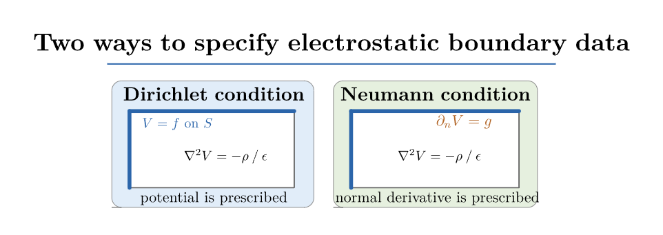
Figure 1. A boundary value problem combines a field equation in the region with boundary data.
Dirichlet data prescribe the potential; Neumann data prescribe its normal derivative.
2 Why a conductor is an equipotential in electrostatic equilibrium
A conductor contains charges capable of moving in response to an applied electric field. If a
nonzero electric field remained inside an ordinary conductor in electrostatic equilibrium, the mobile
charges would continue to move. Electrostatic equilibrium therefore requires
Using E = −∇V gives
Consequently the potential is spatially constant throughout each connected conducting
body:
A conductor is therefore an equipotential object. A conductor may be grounded, maintained at a
prescribed nonzero potential, or electrically isolated. These circumstances impose different global
constraints and must not be treated as interchangeable.
2.1 Tangential electric field at a conducting surface
Take a very short line segment on the surface, with displacement dlt tangent to the conductor.
Because V is constant along the surface,
Then
for every tangent direction, and therefore
At equilibrium, the exterior field immediately adjacent to an ideal conducting surface is normal to
it. This does not mean the exterior field must be everywhere normal to some arbitrarily chosen
coordinate surface; it is normal to the actual conductor boundary.
2.2 The normal field and induced surface charge
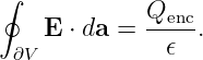
Use a thin Gaussian pillbox straddling the conducting surface. Let its flat end faces have area A,
and choose n to point from the conductor into the surrounding homogeneous dielectric. Gauss’s
Law is
When the pillbox height approaches zero, the curved side contributes negligible flux for a finite
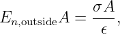
field. The field inside the conductor vanishes. The enclosed surface charge is approximately σA.
Consequently,
so
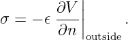
With Equation (3),
This is a key formula: once the potential has been determined, the previously unknown surface
charge can be calculated from its normal derivative.
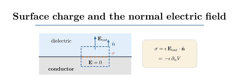
Figure 2. A short Gaussian pillbox crossing an ideal conducting boundary. The interior electric
field vanishes; the normal exterior field is related to surface charge by σ = 𝜖En.
2.3 Boundary conditions across an ordinary dielectric interface
The conductor boundary condition is a special case of two general electromagnetic boundary
conditions. In electrostatics, ∇× E = 0 gives
where the normal points from medium 1 toward medium 2. Gauss’s law for the electric
displacement D = 𝜖E gives
where σf is the free surface charge density. A conductor at electrostatic equilibrium has E1 = 0
and D1 = 0, yielding the preceding conductor formulas. Polarization within dielectric materials
requires the more general D notation.
3 The uniqueness theorem: why boundary data matter
The method of images seems at first like a lucky guess. Its validity rests on the uniqueness of the
boundary value problem. We now derive that theorem.
Suppose V 1 and V 2 both solve Poisson’s equation with the same specified charge density ρ in the
same connected region Ω. Their difference is
Subtract the two Poisson equations:
The difference therefore satisfies Laplace’s equation even if the individual potentials satisfy
Poisson’s equation.
3.1 An integral identity obtained from the product rule
Apply the divergence product rule to the vector field u∇u:
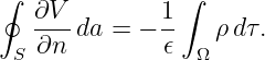
Integrate over Ω:
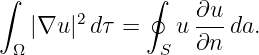
By the divergence theorem, the left side equals a boundary integral:
Using Equation (19) leaves
3.2 Dirichlet uniqueness
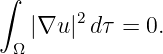
If V 1 and V 2 have the same specified boundary potential, then u = 0 on S. The right side of
Equation (23) is zero:
The integrand is nonnegative. For sufficiently regular solutions it must vanish throughout the
domain:
Therefore u is constant, and its zero boundary value forces the constant to be zero.
Thus
throughout Ω. The electrostatic potential with specified charge density and Dirichlet boundary
data is unique.
3.3 Neumann uniqueness and the additive constant
If instead the normal derivatives agree, then ∂u∕∂n = 0 on S. Again Equation (23) gives ∇u = 0,
so
The electric field is unique, but the potential is only fixed up to an additive constant. Neumann
data must also satisfy a compatibility relation with the volume charge:
This follows immediately by integrating Poisson’s equation and applying Gauss’ theorem.
3.4 Unbounded domains and singular charges
For an unbounded exterior region, a condition at infinity is part of the boundary specification, such
as V → 0 at infinity. A uniqueness proof can be made on a truncated region and then extended to
infinity when the fields decay sufficiently quickly. If an ideal point charge lies in the region, the
solution is singular at that point. To apply the theorem precisely, remove a small neighborhood of
the charge and prescribe its Coulomb singularity, or equivalently work with Poisson’s equation in
the distributional sense.
The practical conclusion is important: once a candidate potential has the correct differential
equation, the correct boundary potential, the prescribed singular charges, and appropriate
behavior at infinity, there is no other solution satisfying all those data.
4 The method of images as a boundary-value construction
An image charge is a mathematical source placed outside the physical solution region in order
to enforce a boundary potential. It is not a second physical charge hidden behind a
conducting wall. The construction is valid only where the actual physical field is being
calculated.
The general procedure is
- Identify the physical region, physical charges, and conductor boundaries.
- Propose one or more mathematical image charges outside the physical region.
- Use Coulomb potentials to satisfy the required boundary values.
- Check Poisson’s or Laplace’s equation everywhere in the physical region, away from
the real charges.
- Check the boundary potential and behavior at infinity.
- Invoke the uniqueness theorem to identify the constructed field with the physical field.
The images reproduce the exterior potential and field; they do not directly describe the
microscopic charges on the conductor. The physical induced charge is obtained afterward using
Equation (15).
5 Point charge above an infinite grounded conducting plane
Place an infinite grounded conductor in the half-space z ≤ 0. The physical field exists in z > 0. A
point charge q sits at (0, 0,a) with a > 0. Grounding imposes
and choose V → 0 at spatial infinity.
Introduce an image charge −q at (0, 0,−a). In z > 0, the candidate potential is
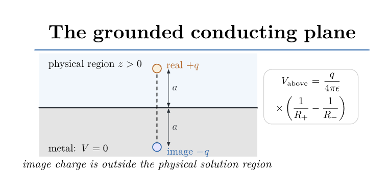
Figure 3. Physical half-space above a grounded conducting plane. The image charge of opposite
sign is located the same distance below the plane and is used only to construct the physical field
above it.
5.1 Proving the plane is an equipotential
Set z = 0. The distances to the real and image charges are equal:
The two terms in Equation (30) cancel and yield
Away from the real charge the potential satisfies Laplace’s equation in z > 0. It also has exactly
the Coulomb singularity of the prescribed charge and tends to zero at infinity. The Dirichlet
uniqueness theorem proves that Equation (30) is the correct physical potential in the upper
half-space.
5.2 The induced surface charge density
Let s =  be the cylindrical radius measured from the point below the charge. Differentiate
Equation (30) with respect to z:
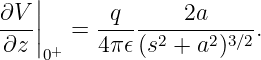
At z = 0+ this reduces to
The outward normal from the conductor is +z. Hence
The induced surface density is negative for a positive charge q and is most concentrated directly
underneath it, where s = 0.
5.3 Total charge drawn from ground
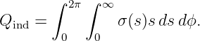
The total induced charge is the surface integral
Inserting Equation (35),
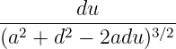
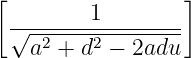
Set u = s2 + a2, so du = 2sds. Then
∫
0∞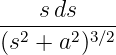 | =  ∫
a2∞u−3∕2 du | |
|
| =  a2∞ | |
|
| =  . | (38) |
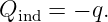
Therefore
The infinite grounded plane draws an amount of charge from the grounding circuit equal and
opposite to the external point charge. This statement refers to the ideal infinite-plane
geometry.
5.4 Force on the physical charge
Although the image is fictitious, its electric field in z > 0 equals the field from the induced
conductor charges. Consequently the force on the real charge can be calculated from the image
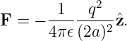
field alone. The charge-image separation is 2a, and the image charge is −q:
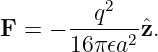
Thus
For either sign of q, the force is attractive toward the conductor.
5.5 Energy and the factor of one half
A frequent mistake is to treat the real and image charges as an ordinary physical two-charge
system and assign the full interaction energy qV image. The induced conductor charge is not held
fixed while the physical charge moves. Its distribution responds continuously to the charge
position.
For a grounded plane, the work-based interaction energy with reference U(∞) = 0 is obtained from
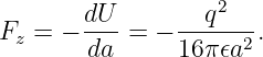
the force:
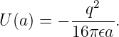
Therefore
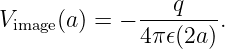
The image potential at the physical charge is
It follows that
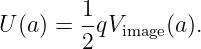
The factor of one half is a consequence of the induced-charge response. It is not a factor applied to
the electric field or to the force.
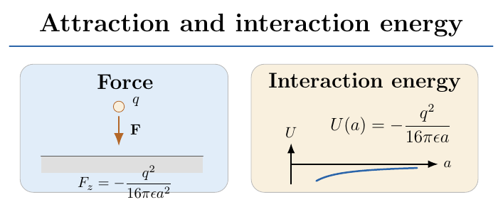
Figure 4. The physical charge is attracted toward the grounded plane. The force is calculated from
the image field; the interaction energy is one half the real-charge times image-potential expression.
6 Grounded conducting sphere with an external point charge
Let a grounded conducting sphere of radius a be centered at the origin. Place a real charge q on
the positive z axis at distance d > a. The physical solution region is exterior to the sphere,
r > a.
We seek an image charge q′ at distance b < a along the same axis, so that
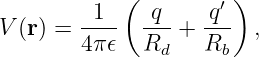
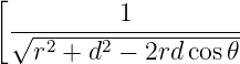
where, at a field point of spherical coordinates (r,𝜃,ϕ),
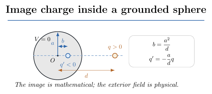
Figure 5. Image-charge construction for a grounded conducting sphere. A physical charge q at
d > a is accompanied mathematically by an image charge q′ at b < a. The conducting boundary is
at r = a.
6.1 Finding the image location and image charge
We want the two distance functions evaluated at r = a to be proportional for every polar angle.
Propose
At the sphere surface,
| Rb2 | = a2 + b2 − 2ab cos 𝜃 | |
|
| = a2 +  −  cos 𝜃 | |
|
| =   | |
|
| =  Rd2. | (50) |
Because distances are positive,
The boundary potential is therefore
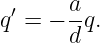
To enforce the grounded boundary condition V (a,𝜃) = 0 for every 𝜃, choose
Thus the complete exterior potential is
Every image lies inside the metal, outside the physical region. The candidate potential satisfies the
required source singularity, has V = 0 at the sphere surface, and decays at infinity. The uniqueness
theorem establishes that it is the physical exterior potential.
6.2 Induced charge distribution on the sphere
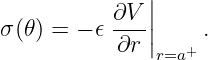
The outward normal from the conductor into the exterior is r. Consequently,
For an arbitrary fixed source position cz,
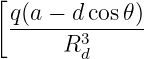
Use Equation (56) in Equation (46):
Substitute b = a2∕d, q′ = −qa∕d, and R
b = (a∕d)Rd. The terms proportional to cos 𝜃 cancel. After
collecting the remaining terms,
For q > 0, the induced surface charge is negative everywhere, with greatest magnitude on the side
nearest the external charge (𝜃 = 0). A grounded sphere may exchange charge with the grounding
connection; its total induced charge need not be zero.
6.3 Total induced charge on the grounded sphere
Directly integrating Equation (58) over the sphere yields
Insert Equation (58), and change variables to
Then
| Qind | = −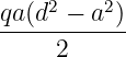 ∫
−11 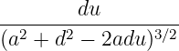 . | (61) |
Differentiate the expression
The derivative is
Therefore
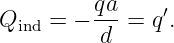
Substituting back gives the exact total induced charge:
An independent check uses Gauss’s law on a very large sphere enclosing both the physical
charge and the conductor. The mathematical far field has the monopole coefficient q + q′,
whereas the physical far field corresponds to q + Qind. The same equality Qind = q′
follows.
6.4 Force and interaction energy
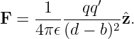
The charge q interacts with the induced conductor charge. Its force equals the force from the image
charge q′ located at b = a2∕d:
Now
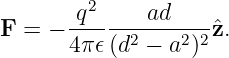
Substituting the image parameters gives
Again the force is attractive for either sign of the physical charge. For a grounded sphere and
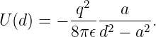
reference U(∞) = 0,
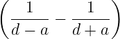
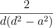
To check, differentiate U with respect to d and verify that Fz = −dU∕dd reproduces
Equation (68). Equivalently U =  qV image(d), evaluated using the image potential at
the real-charge location. As the charge approaches an ideal conducting surface, the
idealized force grows without bound; a realistic microscopic model would eventually be
necessary.
7 A neutral isolated conducting sphere is not a grounded sphere
The grounded-sphere solution has total induced charge −qa∕d. That is not the correct constraint
for an isolated sphere that initially carries zero net charge.
For an isolated neutral sphere, the conducting surface must still be an equipotential,
but its potential is not prescribed to be zero. The required total charge on the sphere
is
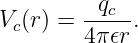
We already have a real-plus-image pair that gives zero potential on the sphere. Add an image
charge qc at the center. The central charge contributes the same potential at every surface point, so
the sphere remains an equipotential. Its extra contribution to the physical exterior solution
is
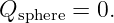
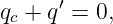
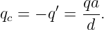
To make the total charge represented by the interior images zero,
so
The exterior potential is then
On r = a the first two terms cancel, leaving
The neutral sphere is therefore generally at nonzero potential relative to infinity.
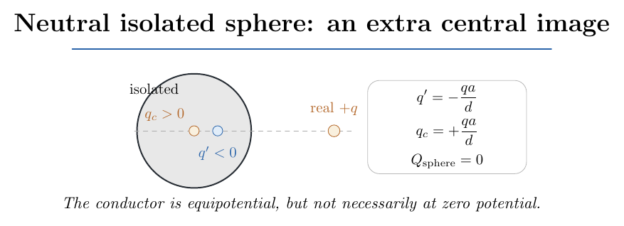
Figure 6. An isolated neutral sphere requires two mathematical images: the off-center image from
the grounded-sphere construction and an additional central image ensuring zero net induced
charge.
7.1 Induced surface density and force for the neutral sphere
By linearity, the neutral sphere’s induced density is the grounded density plus the uniform surface
density from the central image:
Its integral is q′ + qc = 0, as required. The force on the real point charge is the sum of the forces
from the two interior images:
For d ≫ a, expand
The leading a∕d3 contribution cancels the central-image force, leaving
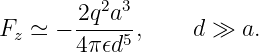
This is the expected far-field induced-dipole attraction. It is weaker at large distances than the
grounded-sphere force, which has a leading d−3 dependence.
7.2 A sphere held at arbitrary potential or with prescribed net charge
A central image of magnitude 4π𝜖aV 0 raises the potential on an initially grounded sphere to the
prescribed value V 0. For this case,
If instead the total physical charge on the isolated conducting sphere is prescribed to be Q0, the
appropriate central image is
These are two different boundary-value specifications. The physical distinction between held
potential and fixed total charge determines which image construction is appropriate.
8 Separation of variables: a method beyond images
The method of images works for special highly symmetric boundaries, but many boundary value
problems require another method. Consider the semi-infinite strip
Suppose the region is charge-free and its boundaries satisfy
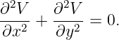
The two-dimensional Laplace equation is
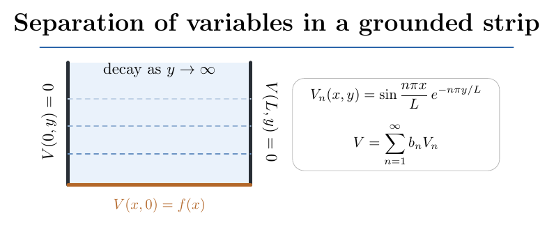
Figure 7. A semi-infinite charge-free strip with grounded side boundaries and prescribed potential
f(x) along the bottom. Separation of variables turns the boundary geometry into sine modes in x
and decaying exponentials in y.
8.1 Step 1: assume a separated product
Try
Substituting into Equation (85),
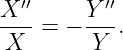
Away from isolated zeros of X and Y , divide by XY :
The left side depends only on x and the right only on y, so both must equal a constant. Choose the
constant −k2 to obtain sine functions in the bounded x direction:
8.2 Step 2: apply the side conditions
The general solution to Equation (89) is
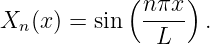
The condition X(0) = 0 requires B = 0. The condition X(L) = 0 then requires
which gives the allowed Wavenumbers
Therefore
8.3 Step 3: select the decaying solution
Equation (90) gives
The field must decay as y →∞, so Cn = 0. Each separated mode is therefore proportional
to
8.4 Step 4: construct the general solution by superposition
Laplace’s equation is linear. Add all the allowed modes:
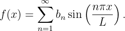
At y = 0, this becomes the Fourier sine series of the prescribed bottom boundary:
Multiply by sin(mπx∕L) and integrate from 0 to L. Orthogonality gives
Consequently
This is an important bridge to the PhysicsLibrary Fourier series sequence: Fourier coefficients are
not merely function approximations. Here they are the amplitudes of spatial modes satisfying the
electrostatic boundary conditions.
8.5 Worked example: one sinusoidal boundary mode
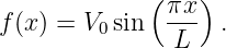
Choose
By orthogonality b1 = V 0 and all other coefficients are zero. Thus
Differentiate to find the electric field:
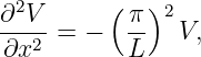
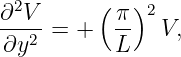
The direct Laplace check is
so their sum vanishes. Each higher sine mode decays more rapidly with y, a useful way to
understand how fine spatial boundary patterns are smoothed at greater distances from the
electrodes.
9 The simplest capacitor as a one-dimensional boundary value problem
Consider two large parallel conducting plates a distance d apart, with negligible edge effects. Let
the lower plate at z = 0 have potential 0 and the upper plate at z = d have potential V 0.
Translation symmetry in the directions parallel to the plates implies V = V (z). Laplace’s equation
becomes
Integrate once:
Integrate a second time:
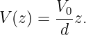
Apply V (0) = 0 to get B = 0. Apply V (d) = V 0 to get A = V 0∕d. Therefore
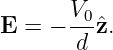
The electric field is uniform:
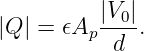
If the plate area is Ap, Gauss’s law gives
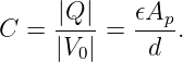
capacitance is the ratio of charge magnitude to potential difference magnitude:
The field-energy density uE =  𝜖E2 gives the total stored energy
| U | =  𝜖E2(A
pd) | |
|
| =   V 02 | |
|
| =  CV 02. | (114) |
This is the boundary-value interpretation of the parallel-plate capacitance formula used in the
EDL04 laboratory.
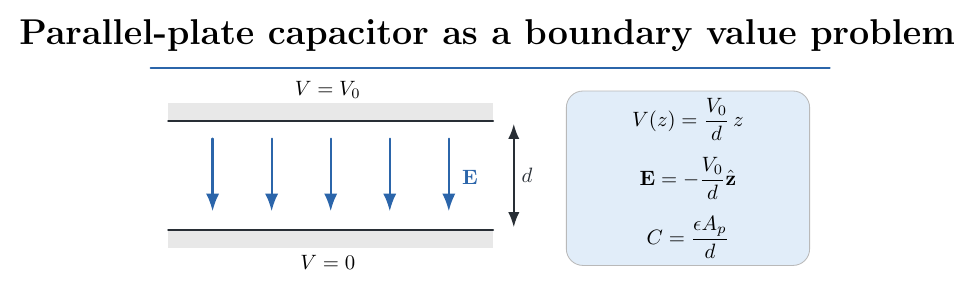
Figure 8. Parallel plates at prescribed potentials produce a linear potential and, away from edge
effects, a uniform electric field. The capacitance follows directly from the normal-field boundary
condition.
10 Numerical boundary value problems and potential mapping
When a conductor has a complicated shape, an analytic image or separated solution may
not exist. The simplest numerical method is based directly on Laplace’s equation. In a
two-dimensional uniform grid with spacing h, approximate the second derivatives by centered
differences:
Setting their sum to zero and solving for the central grid value gives
Thus every interior potential equals the average of its four nearest neighbors, to the accuracy of
this discrete approximation. One can start with an initial guess and repeatedly replace interior
values by this average while keeping prescribed boundary values fixed. Jacobi updates use values
from the previous iteration, while Gauss-Seidel updates can use newly computed values
immediately.
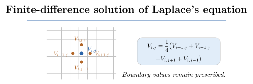
Figure 9. The five-point finite-difference approximation to Laplace’s equation. Interior potential is
constrained by neighboring values, while electrode potentials are imposed on the boundary.
In a grid calculation, convergence is checked from successive solution changes and, preferably, the
residual of the discrete Laplace equation. Near sharp conductor corners the physical field can
be strongly enhanced, so the field obtained by finite differences may converge more
slowly than the potential. Mesh refinement is important when interpreting local field
magnitudes.
10.1 Bridge to EDL03: measuring a potential map
In a low-voltage conducting-paper or resistive-sheet potential-mapping experiment, a meter
measures the scalar voltage V (xi,yj) at sampled locations. Electric-field components are then
estimated by spatial differences:
The conducting sheet realizes a two-dimensional potential problem governed by a current-continuity
equation. In a homogeneous, isotropic sheet with constant conductivity and no interior current
source, the steady potential satisfies Laplace’s equation. It is an effective model for the
mathematics of electrostatics, but the sheet current is not the same physical quantity as free-space
electric displacement. This distinction matters when comparing measured data with electrostatic
field calculations.
11 Worked comparison: what each boundary specification determines
Consider a finite conducting sphere in a charge-free region, with no external charges.
- If the sphere is held at V 0 relative to infinity, the exterior potential is V (r) = aV 0∕r
and the sphere’s net charge is Q = 4π𝜖aV 0.
- If the isolated sphere has prescribed net charge Q, its exterior potential is V (r) =
Q∕(4π𝜖r) when V (∞) = 0, and its surface potential is Q∕(4π𝜖a).
- If the sphere is grounded and there are no external charges, V = 0 throughout the
exterior region.
These cases may have similar mathematics but different physical control variables. The distinction
becomes essential when external charges polarize conductors.
12 Common mistakes and how to avoid them
- Confusing the real conductor surface charge with the fictitious image charge. The image
is a device for reproducing the potential within the chosen region.
- Using the image potential in the wrong physical region. The image solution is
constructed only where it satisfies the real boundary problem.
- Treating a grounded conductor and a neutral isolated conductor as equivalent.
Grounding fixes potential; isolation fixes total charge.
- Applying the normal-derivative formula with the wrong normal direction. For a
conductor the normal used here points from the metal into the exterior.
- Computing force on a real charge from its own Coulomb field. The induced-field
contribution is obtained from the image field, excluding the charge’s singular self-field.
- Omitting the factor of one half when computing image-interaction energy in a grounded
linear electrostatic setup.
- Assuming that a solution of Laplace’s equation is unique without specifying enough
boundary information.
- Applying a separation-of-variables mode expansion without checking the boundary
behavior of every allowed mode.
- Treating a corner singularity in an idealized electrode as a numerical bug. It may be a
genuine feature of an idealized sharp-boundary model.
- Confusing experimental resistive-sheet current with vacuum electric flux, even when
both potential fields satisfy Laplace’s equation.
13 Practice exercises
- From E = −∇V , show directly why a connected ideal conductor must be an
equipotential in static equilibrium.
- Derive the normal-field boundary condition from a Gaussian pillbox and state the
required normal orientation.
- Complete the Dirichlet uniqueness proof for a region with two separate conducting
boundaries, each held at a prescribed potential.
- Derive the Neumann compatibility condition by integrating Poisson’s equation.
- Recalculate the induced density on the grounded plane and verify that it is most
negative at s = 0.
- Integrate the induced plane charge density over a finite disk of radius S and examine
the S →∞ limit.
- From the plane force, calculate the reversible external work to bring a point charge
from infinity to height a.
- Verify the grounded sphere image-location identity Rb = (a∕d)Rd for arbitrary 𝜃 on
the sphere surface.
- Differentiate the grounded-sphere potential to recover Equation (58).
- Integrate the grounded sphere’s induced density explicitly and recover Qind = −qa∕d.
- Find the neutral sphere’s potential at its surface and explain why it differs from zero.
- Expand the neutral-sphere force for d ≫ a and identify the leading power of 1∕d.
- Solve the semi-infinite strip problem for f(x) = V 0 sin(2πx∕L) and check Laplace’s
equation.
- If f(x) is constant between the strip’s corners, calculate the Fourier coefficients and
identify which sine modes survive. Explain why corner limits require care.
- Derive the four-neighbor average rule for a rectangular grid whose horizontal and
vertical spacings are different.
- Use the uniform capacitor solution to derive C = 𝜖Ap∕d and U = CV 02∕2.
14 Summary and preparation for the next article
Electrostatic boundary value problems are governed not just by Coulomb’s law, but by the
combination of a partial differential equation and physically meaningful boundary data.
Conductors are equipotential bodies, their tangential field vanishes, and the normal field
determines surface charge. The uniqueness theorem turns a candidate potential that satisfies the
right conditions into a complete solution.
The method of images exploits symmetry to enforce conductor boundary values without initially
calculating the induced charge distribution. The grounded plane and grounded sphere are two
central examples. Separation of variables and numerical relaxation extend the same physical logic
to more general boundaries.
The natural next step is to develop **ED10: Separation of Variables, Green Functions, and
Multipole Methods for Electrostatic Boundary Value Problems**, including the spherical harmonic
framework and more general geometries.
References
References
[1] D. J. Griffiths, Introduction to Electrodynamics, 5th ed., Cambridge University Press,
2023.
[2] E. M. Purcell and D. J. Morin, Electricity and Magnetism, 3rd ed., Cambridge
University Press, 2013.
[3] J. D. Jackson, Classical Electrodynamics, 3rd ed., Wiley, 1998.
[4] W. R. Smythe, Static and Dynamic Electricity, 3rd ed., McGraw-Hill, 1968.
[5] G. B. Arfken, H. J. Weber, and F. E. Harris, Mathematical Methods for Physicists,
7th ed., Academic Press, 2013.
























 =

![[
− ------z −-a------
[s2 + (z − a)2]3∕2](https://images.physicslibrary.org/cache/objects/1592/make4ht/ElectrostaticBoundaryValueProblemsConductorsAndImageCharges35x.png)
![z + a ]
+ --2---------2-3∕2-
[s + (z + a) ]](https://images.physicslibrary.org/cache/objects/1592/make4ht/ElectrostaticBoundaryValueProblemsConductorsAndImageCharges36x.png)








![]
a∕d
− ∘--2----4--2-------2-------
r + a ∕d − 2ra cos𝜃∕d](https://images.physicslibrary.org/cache/objects/1592/make4ht/ElectrostaticBoundaryValueProblemsConductorsAndImageCharges66x.png)


![q′(a − bcos𝜃) ]
+ -------3------
R b](https://images.physicslibrary.org/cache/objects/1592/make4ht/ElectrostaticBoundaryValueProblemsConductorsAndImageCharges71x.png)