ED08: Electrostatic Fields, Coulomb’s Law, and Superposition
The earlier ED articles established vectors, differential operators, Gauss’ theorem, singular sources,
curvilinear coordinates, and the reconstruction of fields from divergence and curl. We are now
ready to apply those mathematical tools to the first complete physical field model of classical
electrodynamics: the static Electric Field produced by charge.
The theme is to start with the field of one point charge, then build increasingly complicated fields
without changing the underlying law. In each example we distinguish the geometry of the source,
the vector contribution from one source element, and the operation that combines all the
contributions.
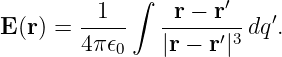
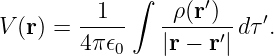
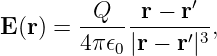
The central vector integral will be
We will derive this expression rather than merely quote it. Its field-point/source-point notation is
intentionally aligned with ED02 and ED07.
1 What electrostatics assumes
Electrostatics treats electric charges whose relevant macroscopic configuration is independent of
time. In the region of interest the electric field is time-independent, and Faraday’s law
gives
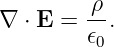
Gauss’s Law gives
The corresponding integral forms are
| ∮
∂V E ⋅ da | =  , | (5)
|
| ∮
CE ⋅ dl | = 0. | (6) |
Coulomb’s law supplies a convenient physical solution for point charges in vacuum. As ED07
emphasized, a field is reconstructed uniquely only after appropriate boundary behavior is also
specified. Throughout the main examples we assume the fields of localized sources approach zero at
spatial infinity, unless stated otherwise.
2 What the electric field measures
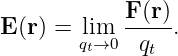
An electric field is operationally defined through the force on a sufficiently small stationary test
charge qt:
The limit expresses the ideal of a probe whose charge is too small to disturb the source
configuration appreciably. It does not mean one must physically use a charge of exactly
zero.
The SI units are
The vector E is independent of the sign of the chosen test charge. A positive test charge
experiences force along E; a negative one experiences force opposite E.
3 Coulomb’s law and the source-to-field vector
For source charge Q at r′ and observation point r, define
| R | = r − r′, | (9)
|
| R | = |R|, | (10)
|
| R | =  . | (11) |
The vector R points from the source to the observation point. This matters: reversing it changes
the sign of the vector formula.
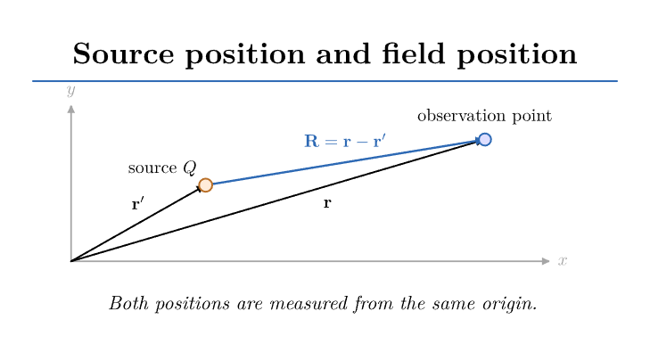
Figure 1. Geometry used in Coulomb’s law. The vector R = r − r′ connects source point to field
point. The source position and observation position are measured from the same origin.
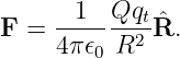
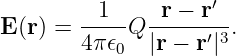
The Coulomb force on the test charge is
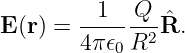
Divide by qt, then take the test-charge limit:
Since R = R∕R,
Two equivalent forms appear frequently:
The first emphasizes the inverse-square magnitude, while the second is often simpler to integrate
component by component.
Checking the sign
For Q > 0, the field points away from the charge. For Q < 0, the vector points toward the charge.
In both cases R still points from the source to the field point; it is the factor Q that reverses the
field direction.
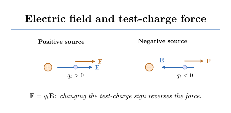
Figure 2. The source-charge sign determines the direction of the electric field; the force on a
negative test charge reverses the direction of the field-force relation.
4 The principle of superposition
Maxwell’s vacuum electrostatic field equations are linear in E and in the source density ρ. If source
1 produces E1 and source 2 produces E2, then
| ∇⋅ (E1 + E2) | =  , | (16)
|
| ∇× (E1 + E2) | = 0. | (17) |
Provided the same appropriate boundary conditions are satisfied, the combined field
is
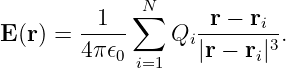
For N point charges,
This is a vector sum. Adding only the magnitudes is incorrect unless every contribution points in
the same direction.
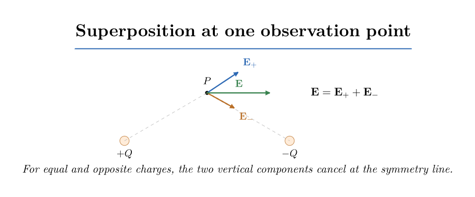
Figure 3. At the same observation point, each charge produces its own electric-field vector. The
physical field is their vector sum, not the sum of their magnitudes.
Step-by-step computational recipe
- Select a single observation point r.
- For every charge i, form Ri = r − ri.
- Evaluate Ri = |Ri|.
- Compute Ei = keQiRi∕Ri3, where k
e = 1∕(4π𝜖0).
- Add Cartesian components or add the vectors in a common orthonormal basis.
- Verify the units, approximate direction, and expected symmetry.
5 From a sum of particles to a charge distribution
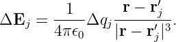
Imagine dividing a finite charge distribution into many small source cells. Cell j contains a small
charge Δqj centered near r′j. Its contribution is approximately
Adding these pieces and refining the partition leads to a continuum integral:
This derivation assumes an integrable source contribution at the observation point. For fields at or
on singular sources, improper integrals, one-sided limits, or distributional treatments may be
needed, as developed in ED05.
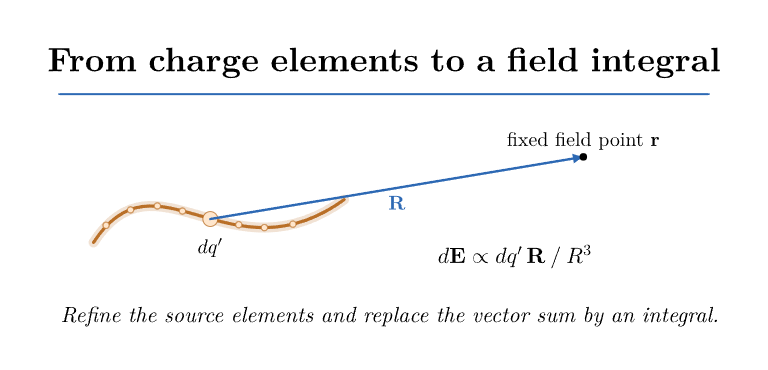
Figure 4. Superposition continues to apply as point charges are replaced by infinitesimal source
elements dq′. Each element has its own source position and separation from the same observation
point.
There are three common density models:
| λ | =  , | dq | = λdℓ, | (22)
|
| σ | =  , | dq | = σ da, | (23)
|
| ρ | =  , | dq | = ρdτ. | (24) |
They have units C∕m, C∕m2, and C∕m3, respectively.
The volume-charge version of Equation (21) is the central result, Equation (2). For a line or a
surface one replaces ρdτ′ by the corresponding λdℓ′ or σ da′.
6 How differential geometry enters the source integral
ED02 and ED06S1 derived the appropriate differential elements from coordinate geometry and the
metric tensor. For example, in cylindrical coordinates,
while in spherical coordinates,
These extra factors are physical volume scalings; they are not optional decorations. The prime
emphasizes that we are integrating over source coordinates. The observation coordinate r remains
fixed during source integration.
A useful separation of responsibilities is:
- the source density describes how much charge lies in a small element;
- the differential element describes the physical size of that element;
- the kernel R∕R3 gives its direction and inverse-square weighting;
- the integral adds all contributions.
7 Electrostatic potential from the Coulomb field
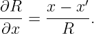
For fixed r′, write R = |r − r′| and calculate a derivative with respect to the observation position
x:
The chain rule gives
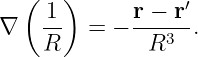
Then
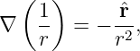
Doing the same for y,z yields the Vector Identity
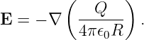
Hence Equation (14) may be written
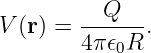
Define the electric scalar potential of the point charge, choosing V → 0 at infinity,
Then
Potential also obeys superposition
Because differentiation and integration are linear,
It is often much easier to integrate 1∕R as a scalar and then differentiate to obtain E than to
integrate three components of R∕R3.
8 The electrostatic field equations follow
For any smooth potential in a source-free region,
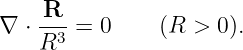
But the point-charge field has a singularity at r = r′. Away from it,
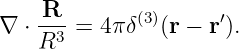
ED05 showed how the missing source appears through a Dirac delta distribution:
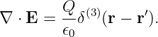
For one charge,
For a continuous density, integrating the identity against ρ(r′) gives
| ∇⋅ E(r) | =  ∫
ρ(r′)δ(3)(r − r′) dτ′ | (40)
|
| =  . | (41) |
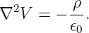
Combining this with E = −∇V produces Poisson’s equation,
In a region without charge,
This is Laplace’s equation. In arbitrary coordinates the scalar Laplacian is replaced by the
Laplace–Beltrami operator derived in ED06S1.
9 How Gauss’s law emerges from the point-charge solution
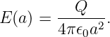
Place a point charge at the center of a sphere of radius a. For Q > 0 the electric field is radial and
has constant magnitude on the sphere,
The outward area element is da = rda. Therefore
| ∮
SE ⋅ da | = E(a) ∮
Sda | (45)
|
| =  (4πa2) | (46)
|
| =  . | (47) |
The factor 1∕a2 in the field cancels the surface-area factor a2. This is why the net flux is
independent of the radius.
For a sphere not centered on a charge, or for an irregular closed surface, the same result follows
from the solid-angle relation dΩ = R ⋅ da∕R2 for an oriented surface. A closed surface has total
oriented solid angle 4π around an enclosed point, and zero around an exterior point. By
superposition we recover Gauss’s law for arbitrary collections of charges and, in the continuum
limit, arbitrary integrable charge distributions.
10 Worked example 1: field on the perpendicular bisector of a finite charged rod
Place a uniformly charged straight segment on the z axis from −L to +L. Let its line charge
density be λ. Evaluate the electric field at r = sx with s > 0.
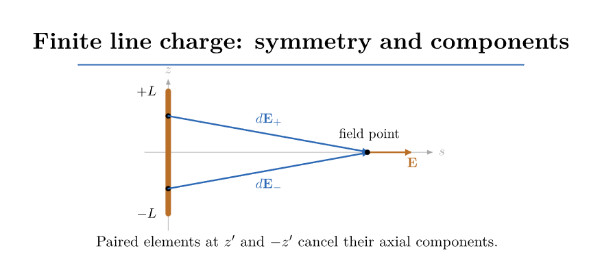
Figure 5. A finite line charge on the z axis. For opposite source elements at z′ and −z′, the
vertical field components cancel and the horizontal components add at the observation point on
the perpendicular bisector.
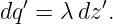
A small rod element contains
The source position is r′ = z′z, so
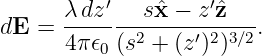
Its field contribution is
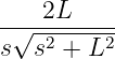
The z component is an odd function of z′, so it integrates to zero over symmetric limits. Only Ex
remains:
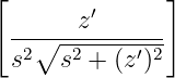
We can derive the needed antiderivative by differentiating
Thus
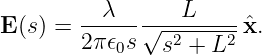
Our final vector result is
For a positive λ, it points away from the rod. The expression is valid for s > 0.
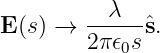
Infinite-line limit
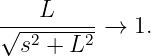
As L →∞ while s stays fixed,
Hence
This is also the result of a cylindrical Gaussian surface. Notice the field scales as 1∕s for an infinite
line, not 1∕s2, because the geometry of the distributed source differs from that of a point
charge.
11 Worked example 2: field along the axis of a charged ring
Place a uniformly charged ring of radius a in the xy plane with total charge Q. Find the field on its
axis at (0, 0,z).
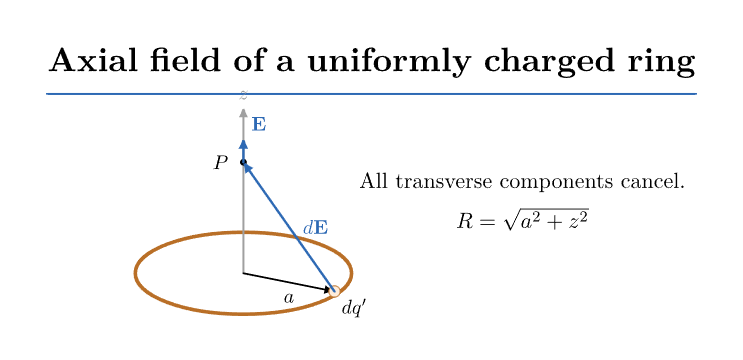
Figure 6. A source element on a uniformly charged ring contributes a field vector toward the
observation point. The transverse components cancel after integrating around the full ring; only
the axial component survives.
Parameterize the source position as
The separation is
and its magnitude is independent of ϕ′:
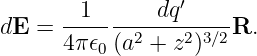
The field element is
Because charge is uniform around the ring, integration of cos ϕ′ and sin ϕ′ over one revolution gives
zero. The remaining component is
Since ∫
dq′ = Q,
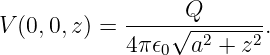
The potential is even simpler, because every source element has the same distance from the field
point:
Differentiate as a check:
At the center z = 0, the net field is zero but the potential is generally not zero. That distinction is
important.
12 Worked example 3: disk built from concentric rings
Let a thin disk of radius a lie in the xy plane with uniform surface charge density σ. Find the field
at height z > 0 on the axis.
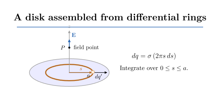
Figure 7. A uniformly charged disk is decomposed into concentric rings. The ring formula is
reused after replacing its charge by dq = σ(2πsds).
One differential ring has radius s and width ds. Its area is
so its charge is
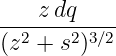
Using the axial field of a ring from Equation (63),
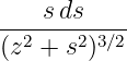
Integrate over 0 ≤ s ≤ a:
Let u = z2 + s2, so du = 2sds. Then
∫
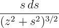 | =  ∫
u−3∕2du | (71)
|
| = −u−1∕2 | (72)
|
| = − . | (73) |
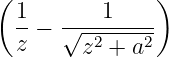
For z > 0,
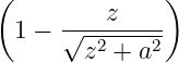
Therefore,
Infinite-plane limit
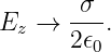
With z > 0 fixed, let a →∞:
For the ideal infinite sheet the field is uniform on each side, with opposite directions
above and below for σ > 0. The discontinuity across the sheet is consistent with the
pillbox boundary condition derived in ED04 and the distributional source ρ = σδ(z) from
ED05.
13 Worked example 4: spherical shell and uniformly charged solid sphere
Spherical symmetry is a case where Gauss’s law gives a shorter derivation than direct integration
of the Coulomb kernel. We should nevertheless understand the limits of this shortcut: the
charge density must be spherically symmetric, not merely contained somewhere inside a
sphere.
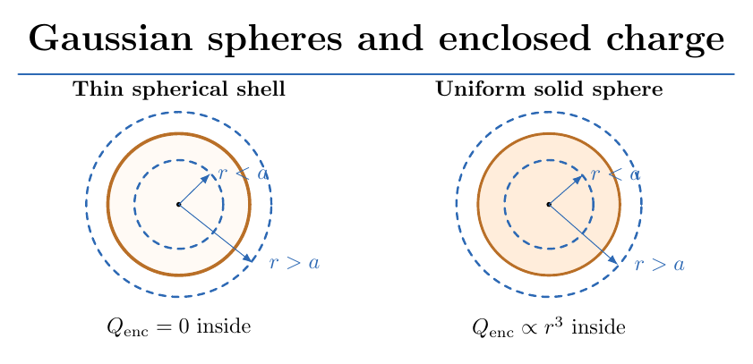
Figure 8. Spherical Gaussian surfaces inside and outside a uniformly charged sphere. For a shell or
solid sphere, spherical symmetry makes the electric field radial and constant in magnitude over
each Gaussian surface.
Thin spherical shell
For a uniformly charged infinitesimally thin spherical shell of radius a and total charge Q, spherical
symmetry implies E = E(r)r. Gauss’s law gives
For 0 < r < a, the enclosed charge is zero, so E = 0. For r > a, Qenc = Q, so
The field jumps across the charged shell. Its limiting values differ by σ∕𝜖0 in the outward Normal
component, where σ = Q∕(4πa2).
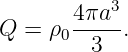
Uniform solid sphere
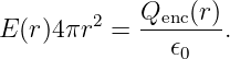
Let a solid sphere of radius a have constant volume density ρ0:
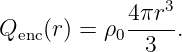
For 0 ≤ r < a, the enclosed charge is
Then
| E(r)4πr2 | =  , | (82)
|
| E(r) | =  . | (83) |
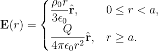
For r ≥ a, the field is that of a point charge Q at the center. Therefore
Derive the potential inside the solid sphere
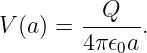
Choose V (∞) = 0. Outside, V (r) = Q∕(4π𝜖0r). At the surface,
For any r < a, using Er = −dV∕dr,
The integral is elementary:
| V (r) − V (a) | = −  ar | (87)
|
| =  (a2 − r2). | (88) |
Using ρ0 = 3Q∕(4πa3), we get
At r = a the inside expression agrees with the outside expression. Its radial derivative also
matches because there is no additional surface delta charge at the boundary of this volume
distribution.
14 A first multipole approximation: the electric dipole
Consider two charges +q and −q at r+ = d∕2 and r− = −d∕2, respectively. The dipole moment
is
pointing from the negative charge to the positive charge.
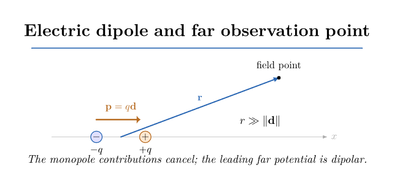
Figure 9. The dipole moment points from negative to positive charge. Far from the pair, the
leading nonzero potential varies as 1∕r2, not 1∕r.
Superposition gives the exact potential
For r ≫|d|, Taylor-expand the kernel:
Because
we obtain
Applying this once with a = +d∕2 and once with a = −d∕2, the two monopole terms 1∕r cancel.
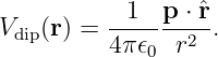
To leading nonzero order,
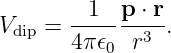
Since p ⋅r = (p ⋅ r)∕r,
To obtain its field, differentiate using the product rule:
∇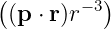 | = pr−3 + (p ⋅ r)∇(r−3) | (97)
|
| =  − 3  . | (98) |
Therefore
The far field of a dipole decreases as 1∕r3. This is an approximation for r ≫|d|, not an exact
expression for finite charge separation.
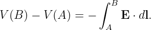
15 Work, potential difference, and the sign convention
For a quasistatic displacement of a test charge qt through a fixed electrostatic field, the electric
force performs differential work
Electrostatic potential energy changes by the negative of the field’s work:
Writing U = qtV for a fixed test charge,
Consequently,
The electrostatic field points in the direction of decreasing V . A negative charge experiences
force opposite E and can accelerate toward greater V while its potential energy qtV
decreases. Keeping force, potential, and potential energy separate prevents common sign
mistakes.
16 Worked numerical example: two charges and a field-point calculation
Let Q1 = +2.0 nC at (0, 0, 0) and Q2 = −1.0 nC at (0.10, 0, 0) m. Find the electric field and
potential at P = (0, 0.10, 0) m in vacuum.
First form the source-to-field vectors,
| R1 | = (0, 0.10, 0) m, | (104)
|
| R2 | = (−0.10, 0.10, 0) m. | (105) |
Their magnitudes are
Using ke ≃ 8.99 × 10⁹ N m2∕C2,
| E1 | = ke y = (1798 N∕C)y, | (107)
|
| E2 | = ke . | (108) |
For the negative second charge the field points from P toward Q2, along (+x −y)∕ . Its
magnitude is 449.5 N∕C, so
Adding components,
Potential is scalar, so
| V (P) | = ke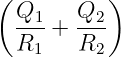 | (111)
|
| ≃ (179.8 − 63.6) V | (112)
|
| ≃ 116.2 V. | (113) |
The field vectors add componentwise, while the potentials add as signed scalars. Both calculations
use the same source geometry.
17 When superposition is not enough by itself
Superposition is a statement about linear field equations for a specified source distribution. In a
real electrostatic experiment the charge distribution can itself change when another Conductor,
dielectric, or charged object is introduced.
For example, placing a neutral conductor near a charged object induces redistribution of surface
charge. The original source density is no longer the same. The total field still obeys Coulomb
superposition over the new combined charge distribution, but one cannot simply add fields
computed from source models that ignore the induced charges.
Other caveats include:
- ideal point, line, and sheet charges are singular mathematical models;
- material polarization modifies the relation between free charge and field;
- nonlinear constitutive materials can invalidate naive superposition of separately solved
material states;
- time-dependent sources require the full Maxwell equations and retardation, not an
instantaneous Coulomb integral.
18 Laboratory bridge: what can be measured?
EDL02 explores static charge and electrostatic forces, while EDL03 maps a scalar potential
using a probe on a conductive sheet. These experiments connect to ED08 in different
ways.
A voltage probe measures a potential difference between its terminals, not E directly. For a
sufficiently fine two-dimensional measurement grid, the electric-field components can be estimated
from
| Ex(x,y) | ≃− , | (114)
|
| Ey(x,y) | ≃− . | (115) |
This is a discrete version of E = −∇V from ED03. The approximation improves with grid
refinement until instrument noise, contact resistance, and probe disturbance become
important.
A controlled measurement workflow is:
- Define the source configuration and its symmetry.
- Record probe coordinates and voltage reference.
- Measure V on a grid, not just at isolated locations.
- Estimate the field vector from neighboring potential samples.
- Check whether the inferred field is nearly perpendicular to equipotential contours.
- Compare the measured field pattern with a simple analytic or numerical source model.
The conductive-sheet experiment is an analogy for electrostatic potential solving, not a direct
measurement of a three-dimensional free-space Coulomb field. Its boundaries and sheet
conductivity matter.
19 Dimensional and limiting checks
Any field derived from a source integral should pass several tests:
- A point-charge field has units N∕C and scales as Q∕r2.
- A finite segment far from the rod looks approximately like a point charge with total
charge 2λL.
- A ring at |z|≫ a looks like a point charge with total charge Q.
- The disk field for a ≫ z > 0 approaches the infinite-plane result.
- A uniformly charged sphere has a finite field at its center and matches the external
inverse-square field at its surface.
- If a distant source has zero total charge, the leading 1∕r potential term may cancel,
exposing dipole or higher multipole behavior.
20 Practice problems
- Starting from the scalar Coulomb magnitude, derive Equation (14) and explain every
factor of R.
- Two equal positive charges lie at x = ±a. Find E at the origin and the potential there.
- Place +Q at x = a and −Q at x = −a. Find the electric field at the origin and verify
the direction.
- Derive the far-distance limit of Equation (55) at fixed L and compare with a point
charge Q = 2λL.
- Use the potential integral to obtain V (s) on the perpendicular bisector of the finite
rod. Set V (∞) = 0.
- Differentiate the ring potential and recover Equation (63).
- Find the value of z > 0 where the axial ring field has its maximum magnitude for
Q > 0.
- Integrate the disk field in z to obtain the on-axis potential for z > 0 with V (∞) = 0.
- Derive the interior potential of a uniformly charged spherical shell and explain why it
is constant.
- Verify continuity of V and of Er at r = a for the uniformly charged solid sphere.
- Derive the far-field dipole potential using a first-order Taylor expansion of 1∕|r − a|.
- Show that an idealized nonzero constant electrostatic field cannot satisfy E → 0 at
infinity, even though its divergence and curl vanish.
- Use centered differences on a simple grid V (x,y) = V 0 − αx2 − βy and compare the
estimated field with −∇V .
- Explain why an image-charge solution for a conductor does not imply the conductor
carries the image charge at the image location.
21 Summary and next step
The point-charge vector field,
extends by superposition to sums and source integrals. The same geometry generates the scalar
potential kernel 1∕R, and the identity E = −∇V connects potential measurements to force per
unit charge.
Gauss’s law, Poisson’s equation, and Coulomb’s law are mutually consistent descriptions of
electrostatics when distributions and boundary conditions are handled correctly. Symmetry and
dimensional analysis help choose which representation is easiest for a given physical
problem.
The natural continuation is ED09: Electrostatic Boundary Value Problems, Conductors, and Image
Charges, where conductor boundaries and induced charges become central rather than secondary
complications.
References
References
[1] D. J. Griffiths, Introduction to Electrodynamics, 5th ed., Cambridge University Press,
2023.
[2] E. M. Purcell and D. J. Morin, Electricity and Magnetism, 3rd ed., Cambridge
University Press, 2013.
[3] J. D. Jackson, Classical Electrodynamics, 3rd ed., Wiley, 1999.
[4] H. M. Schey, Div, Grad, Curl, and All That, 4th ed., W. W. Norton, 2005.