ED07: Helmholtz Decomposition, Potentials, and Field Reconstruction
The vector field F(r) may vary in both magnitude and direction throughout space. ED03
introduced its divergence and curl; ED04 explained their integral meanings; ED05 established the
correct treatment of singular sources; and ED06 derived the differential operators in
symmetry-adapted coordinates. A natural question now arises:
Under suitable decay, regularity, boundary, and topological assumptions, the answer is yes. The
result is called the Helmholtz decomposition theorem. In free space it splits a sufficiently
well-behaved vector field into an irrotational part and a solenoidal part:
The scalar potential Φ and vector potential A are computed from the field’s divergence and curl.
This is a mathematical explanation for why potentials are so central to electrodynamics, not
merely a convenient guessing method.
The words under suitable assumptions matter. On finite domains, boundary data are essential; in
multiply connected regions, circulation around holes can carry information that neither local
divergence nor local curl contains. We will derive the reconstruction, show the failure modes, and
connect everything to electric and magnetic fields.
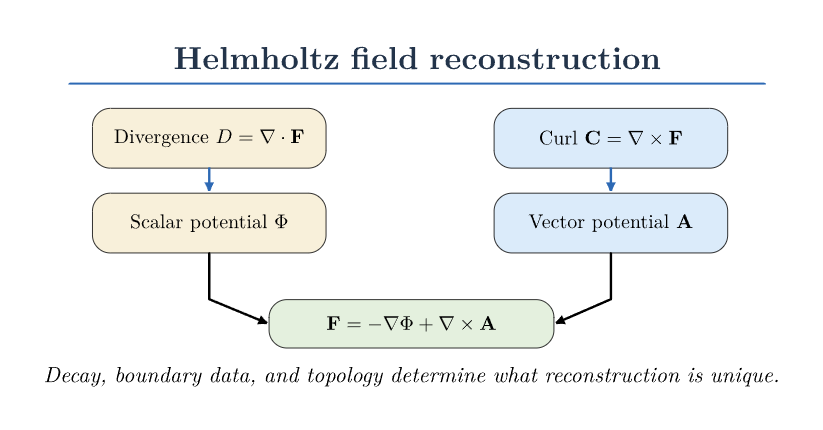
Figure 1. Divergence and curl encode complementary local information. Together with the
appropriate decay, boundary, and global circulation information, they determine a vector field.
1 First distinguish two kinds of field structure
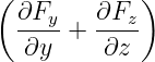
The divergence is a scalar field,
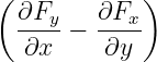
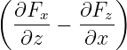
while the curl is a vector field,
Because a divergence of a curl is identically zero,
Thus the three components of C cannot be specified independently: they must satisfy this
compatibility condition. Likewise, on a bounded domain the divergence source and the prescribed
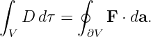
outward Normal field must satisfy the divergence theorem,
Call a field irrotational if ∇× F = 0, and solenoidal if ∇⋅ F = 0. An irrotational field need not be
constant. A solenoidal field need not circulate visibly around circular streamlines. These are
differential properties, not pictures alone.
2 A vector identity provides the starting point
For a twice differentiable vector field the vector Laplacian obeys
Here ∇2F means applying the scalar Cartesian Laplacian to each Cartesian component of F.
Rearranging gives
Insert Definitions (3) and (4):
This is already close to a reconstruction equation. It says that the componentwise Laplacian of the
unknown field is fixed by derivatives of its divergence and curl.
A component-level check
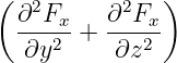
For the x component, the curl of the curl is
Expand and group the mixed derivatives:
Adding and subtracting ∂2F
x∕∂x2 yields
The y and z components follow by cyclic permutation. This gives a direct derivation of
Equation (7) instead of treating it as a mnemonic.
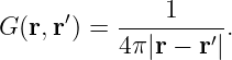
3 Review: the Green function for Poisson’s equation
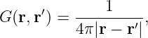
The free-space Green function is
The coordinate r′ identifies a source point; r identifies the field or observation point.
Define
The distributional identity from ED05 is
Thus the solution of
that decays appropriately at infinity is
Indeed, acting with the Laplacian and using the delta sifting property gives
| ∇2u(r) | = ∫
(∇2G)s(r′) dτ′ | (18)
|
| = −∫
δ(3)(r − r′)s(r′) dτ′ | (19)
|
| = −s(r). | (20) |
This solution is particular to free space. If a boundary is present, one must impose boundary data
or add an appropriate harmonic correction.
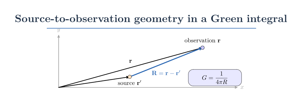
Figure 2. Green-function reconstruction sums contributions from source points r′ to the
observation point r, weighted by G = 1∕(4πR). The integration is over three-dimensional source
volume.
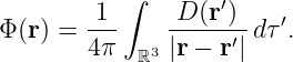
4 Construct a scalar potential from divergence
Given D = ∇⋅ F, define
Equation (15) immediately gives
The associated gradient field
is irrotational because ∇×∇Φ = 0, and it has the required divergence:
| ∇⋅ FL | = −∇2Φ | (24)
|
| = D. | (25) |
The subscript L stands for longitudinal. In Fourier space the gradient points along the wave vector,
giving the name its precise meaning.
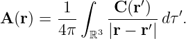
5 Construct a vector potential from curl
Given C = ∇× F, define the vector potential component by component:
The same Green-function identity gives
Now show why this particular potential is divergence-free. In the integral,
Therefore
| ∇⋅ A | = ∫
C(r′) ⋅∇Gdτ′ | (29)
|
| = −∫
C(r′) ⋅∇′Gdτ′. | (30) |
Use the product rule in the source coordinates:
Then
| ∇⋅ A = | −∮
S∞GC ⋅ da′ | |
|
| + ∫
G(∇′⋅ C) dτ′. | (32) |
For localized, sufficiently decaying sources the surface term vanishes. The remaining volume term
vanishes by Equation (5). Consequently
This is the Coulomb gauge. It emerges automatically for the free-space integral in Equation (26)
under these assumptions.
Define the transverse field
Its divergence is identically zero:
Its curl is
| ∇× FT | = ∇× (∇× A) | (36)
|
| = ∇(∇⋅ A) −∇2A | (37)
|
| = C. | (38) |
So FT reproduces exactly the prescribed curl.
6 Put the two contributions together
Define
Take its divergence:
| ∇⋅ Frec | = −∇2Φ + ∇⋅ (∇× A) | (40)
|
| = D + 0 = D. | (41) |
Take its curl:
| ∇× Frec | = −∇×∇Φ + ∇× (∇× A) | (42)
|
| = 0 + C = C. | (43) |
Thus F and Frec have identical divergence and curl. Their difference
satisfies
The Vector Identity then implies
Every Cartesian component is harmonic. In all of ℝ3, if H is smooth, bounded, and tends to zero
at infinity, the maximum principle (or Liouville’s theorem for harmonic functions) gives H = 0.
This proves the free-space reconstruction:
with Φ and A given by Equations (21) and (26). More delicate versions of the theorem cover other
decay classes and distributional sources; the formulas should not be applied indiscriminately to
growing or non-decaying fields.
7 A second proof using the vector Poisson equation
We can also derive the decomposition directly from Equation (9). Formally invert its Laplacian
with the free-space Green function:
Substitute ∇r′2F = ∇′D −∇′× C:
| F(r) = | −∫
G∇′D dτ′ | (49)
|
| + ∫
G(∇′× C) dτ′. | (50) |
Integrate by parts, assuming the terms at infinity vanish. For the first integral,
| ∫
G∇′D dτ′ | = −∫
D∇′Gdτ′ | (51)
|
| = ∇∫
GD dτ′ = ∇Φ. | (52) |
For the second, use ∇′× (GC) = ∇′G × C + G∇′× C. The surface term again vanishes,
leaving
| ∫
G∇′× Cdτ′ | = −∫
∇′G × Cdτ′ | (53)
|
| = ∇×∫
GCdτ′ | (54)
|
| = ∇× A. | (55) |
Therefore the inversion reproduces Equation (47). This proof explains structurally why both a
gradient and a curl appear. The first proof established that they reproduce the prescribed
local data; this one reconstructs them from the Green-function inverse of the vector
Laplacian.
8 Why the names longitudinal and transverse?
For a Fourier component with nonzero wave vector k, write
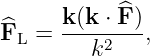
as one mode in a Fourier superposition. On that mode, ∇ acts as ik. Define the parallel
projection
and the perpendicular remainder
These satisfy
The divergence and curl Fourier coefficients are
Solving for the two projections gives
The zero-wave-number mode is not captured by division by k2; it is precisely where constants and
other global or boundary information matter.
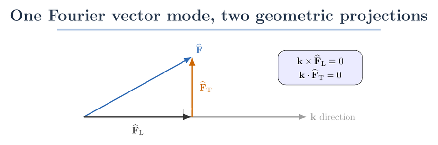
Figure 3. Relative to a Fourier wave vector k, a vector mode separates into a longitudinal
projection parallel to k and a transverse projection perpendicular to k.
9 Potentials and gauge freedom
The vector field in Equation (47) is unchanged by the transformation
for any sufficiently regular scalar χ, since
This is gauge freedom. The particular free-space reconstruction above chooses a divergence-free
vector potential. If a different vector potential is given, it can be adjusted to Coulomb gauge by
solving
The scalar potential is unchanged under an additive constant because its gradient does not depend
on that constant. These familiar freedoms should not be confused with ambiguity in the
physical field: gauge transformations change the potentials but not the reconstructed
field.
In Electromagnetism with time-dependent fields, the physical potentials have the larger gauge
transformation
That dynamical gauge freedom will be treated in a later ED article. The scalar and vector
potentials in the purely spatial Helmholtz theorem need not equal the retarded electromagnetic
potentials.
10 Electrostatics: the scalar potential becomes physical
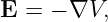
For an electrostatic electric field,
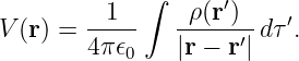
In all of space, assuming suitable decay and no additional boundary field, Helmholtz reconstruction
gives
with
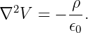
Applying the Laplacian yields Poisson’s equation,
Thus the standard electrostatic potential is a direct specialization of the scalar part of
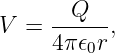
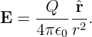
Helmholtz decomposition. For a point charge Q at the origin, the ED05 delta distribution
yields
and therefore, for r > 0,
This satisfies Gauss’s Law distributionally at the origin.
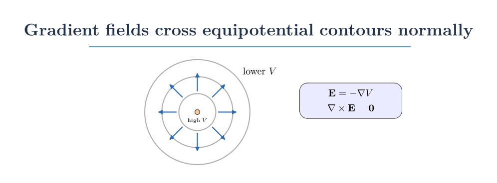
Figure 4. An electrostatic field is normal to equipotential contours and is locally curl-free. The
scalar potential retains source and boundary information that field lines alone do not show.
11 Magnetostatics: the vector potential becomes physical
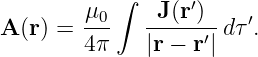
For steady, localized currents in free space,
The continuity equation for stationary sources gives
as required by the compatibility condition for a curl. Helmholtz reconstruction sets the scalar
contribution to zero when ∇⋅ B = 0 and the field decays properly, giving
where
Taking the curl and using ∇G = −∇′G gives
| B(r) | =  ∫
∇  × J(r′) dτ′ | (76)
|
| =  ∫  dτ′. | (77) |
This is the volume-current Biot-Savart expression. Helmholtz decomposition therefore connects
Ampere’s differential law to the Biot-Savart field integral, under the assumptions of magnetostatics
and free space.
12 Worked example 1: a smooth, localized gradient field
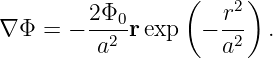
Let
Here r2 = x2 + y2 + z2. First differentiate the exponent:
Thus
Set
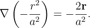
Because it is a gradient, its curl vanishes everywhere. Find its divergence with the product
rule:
| ∇⋅ F | =  ∇⋅  | (82)
|
| =   | (83)
|
| =  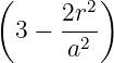 e−r2∕a2
. | (84) |
The divergence is positive near the origin and negative sufficiently far away, while the field decays
rapidly. Its total divergence integrates to zero, consistent with zero net flux at infinity.
Reconstructing from Equation (21) recovers the original Φ up to an additive constant,
fixed here by Φ → 0 at infinity. This is a convenient smooth example without point
singularities.
13 Worked example 2: a smooth, localized solenoidal field
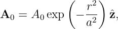
Choose a simple vector potential in Cartesian coordinates,
with constant A0. Its curl is
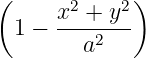
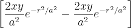
This field loops around the z axis and decays rapidly in every spatial direction. The divergence
is
| ∇⋅ F | =   | (87)
|
| =   | (88)
|
| = 0. | (89) |
Let K = 2A0∕a2 and g = e−r2∕a2. The curl of Equation (86) is
The field is solenoidal, but its curl is nonzero. The free-space Helmholtz integral reconstructs it
entirely from Equation (90) and the decay condition. The convenient trial potential A0 is not
necessarily in Coulomb gauge; different potentials producing the same F may differ by a
gradient.
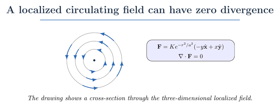
Figure 5. A smooth solenoidal field may wrap around an axis, have nonzero curl, and decay in all
directions. Divergence measures net local flux, not whether nearby field lines visually curve.
14 Worked example 3: a constant field cannot be reconstructed from local data alone on a
ball
Let V be a spherical region and define
Both satisfy
throughout the ball. They are nevertheless different physical fields. The difference is the nonzero
harmonic field E0x.
The boundary normal component distinguishes them. On a sphere of radius R,
where 𝜃 is polar angle measured from +z and ϕ is azimuth. For F1 the normal component is zero.
Thus specifying only divergence and curl does not fix this finite-domain problem; the boundary
field is additional data.
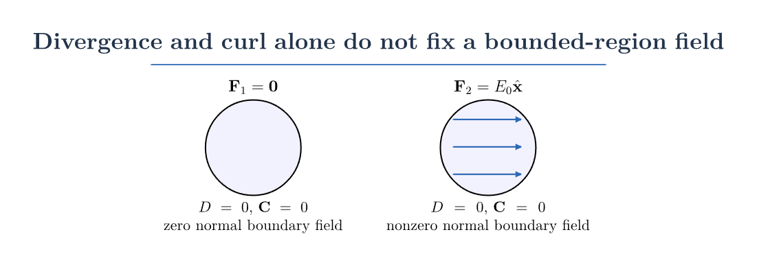
Figure 6. Two fields inside the same finite ball share zero divergence and curl but differ in
boundary-normal data. The missing information is not captured by the local differential operators
alone.
15 Uniqueness with suitable normal boundary data
Suppose F1 and F2 have the same divergence, curl, and normal component on the boundary of a
connected, simply connected region V with sufficiently smooth boundary. Their difference H
satisfies
In a simply connected region, curl-free H can be represented by a single-valued scalar
function:
The divergence condition becomes Laplace’s equation,
The boundary condition is
Now integrate the divergence identity
over V . The divergence theorem gives
| ∫
V |∇ψ|2 dτ | = ∮
∂V ψ da −∫
V ψ∇2ψ dτ | (99)
|
| = 0. | (100) |
The integrand |∇ψ|2 is nonnegative, so it must vanish everywhere for smooth ψ. Consequently
∇ψ = 0, hence F1 = F2. This proves uniqueness for the specified simply connected finite-domain
setting. Existence additionally requires compatible source and boundary data; uniqueness by itself
does not guarantee a solution exists.
16 Topology: a field around a hole can escape the local tests
Consider the annular cylindrical region
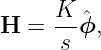
Define
where K is constant. Throughout this region, the cylindrical divergence is
and the z component of its curl is
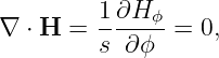
| (∇× H)z | =   (sHϕ) | (104)
|
| =   = 0. | (105) |
The other curl components also vanish. The field is tangent to the inner cylinder, outer cylinder,
and flat end caps, so
Nevertheless the circulation around a loop of fixed s and z is
| ∮
CH ⋅ dl | = ∫
02π (sdϕ) | (107)
|
| = 2πK. | (108) |
This is nonzero when K≠0. The same local divergence, curl, and normal boundary data are also
satisfied by 0. Here the domain has a hole, so the previous simply connected uniqueness
proof does not apply. The circulation around a noncontractible loop supplies additional
information.
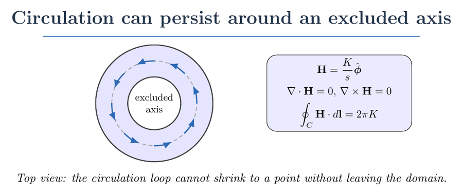
Figure 7. In an annular region, Kϕ∕s has zero divergence, zero ordinary curl, and zero normal
boundary component, yet nonzero circulation around the excluded axis. A global circulation
period distinguishes it from the zero field.
If one extends Equation (102) to all space including the axis, it becomes singular there. ED05
showed the corresponding distributional curl is concentrated on the axis, so the local zero-curl
claim must be restricted to s > 0. This example connects the topology of a hole with the
singular-source mathematics of the previous lessons.
17 Finite-domain Green representations and boundary information
Why did the free-space integral omit boundary information? The simplest explanation comes from
Green’s second identity applied to each Cartesian component Fi. With
and r inside a bounded volume V , the component Green representation is
| Fi(r) = | −∫
V G∇r′2F
i dτ′ | |
|
| + ∮
∂V 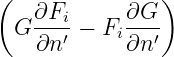 da′. | (110) |
The volume term contains ∇′D −∇′× C by Equation (9). The surface term contains information
about the field and its derivatives on the boundary. This does not mean both quantities must be
specified independently: boundary-value problems prescribe suitable data, and the equations
determine the rest. It means that the interior source data alone are generally insufficient for
reconstruction on a finite region.
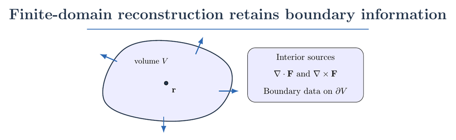
Figure 8. For a finite region, source information in the interior must be accompanied by suitable
boundary information. Green’s representation separates volume and boundary contributions
explicitly.
18 A caution about time-dependent electrodynamics
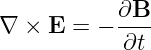
At a single instant, the Helmholtz theorem may be applied mathematically to E(r,t) or B(r,t) as
a spatial field, under the same spatial assumptions. But the resulting instantaneous
potentials are not by themselves a causal solution of Maxwell’s dynamical equations. In
particular,
means the electric field need not be purely longitudinal. Physical retarded potentials, gauge
conditions, and initial radiation data must be handled in the full time-dependent problem. Avoid
interpreting the free-space Helmholtz integrals at each time as propagation rules with infinite
signal speed.
19 Practical field-reconstruction workflow
When given divergence, curl, or measured field data:
- State the spatial domain. Is it all space, a finite simply connected volume, or a region
with holes?
- Check compatibility: ∇⋅ C = 0 and any boundary flux constraints.
- Specify decay behavior at infinity or appropriate boundary conditions.
- For full space, construct Φ from D and A from C using the Green integrals.
- Reconstruct F = −∇Φ + ∇× A.
- Verify both divergence and curl; then verify the boundary conditions or decay.
- In multiply connected domains, check circulation around independent noncontractible
loops.
- For singular fields, interpret the differential identities distributionally and inspect
excluded points, lines, or surfaces.
This workflow turns a formal theorem into a practical method for electromagnetics and
computational field modeling.
20 Practice exercises
- Starting from the component definition of curl, verify Equation (7) for the y
component.
- Given D(r) and C(r), write the two free-space potential integrals and list their decay
assumptions.
- Starting from Equation (26), show carefully that ∇⋅ A = 0 when ∇⋅ C = 0 and all
surface terms vanish.
- Show that ∇⋅ (∇× A) = 0 and ∇×∇Φ = 0 wherever the potentials are sufficiently
smooth.
- Verify Equation (84) independently in spherical coordinates.
- Verify ∇⋅ F = 0 for the localized vortex in Equation (86) using Cartesian partial
derivatives.
- In Equation (85), compute ∇⋅ A0 and explain why the trial potential is not generally
in Coulomb gauge.
- Let F = F0z inside a finite ball. Find D, C, and F ⋅n on its surface.
- Show directly that the circulation in Equation (108) does not depend on the loop
radius s.
- Derive the free-space electrostatic scalar potential by setting D = ρ∕𝜖0 and C = 0.
- Starting with the steady-current vector potential, take its curl to obtain the Biot-Savart
integral.
- For k = (k, 0, 0), show explicitly which Cartesian components of a Fourier vector mode
are longitudinal and which are transverse.
21 Summary
The vector identity
reveals why divergence and curl are the source data for the vector Poisson problem. Under
appropriate free-space assumptions,
with
and
The first field part is longitudinal and curl-free; the second is transverse and divergence-free.
Electrostatic and magnetostatic potentials arise as the corresponding special cases. On finite or
multiply connected domains, boundary data and global circulation information are essential to a
correct uniqueness statement.
References
[1] D. J. Griffiths, Introduction to Electrodynamics, 5th ed., Cambridge University Press,
2023.
[2] H. M. Schey, Div, Grad, Curl, and All That, 4th ed., W. W. Norton, 2005.
[3] G. B. Arfken, H. J. Weber, and F. E. Harris, Mathematical Methods for Physicists,
7th ed., Academic Press, 2013.
[4] J. D. Jackson, Classical Electrodynamics, 3rd ed., Wiley, 1998.
[5] P. M. Morse and H. Feshbach, Methods of Theoretical Physics, McGraw-Hill, 1953.