ED04: Gauss’s Theorem, Stokes’ Theorem, and Integral Field Laws
ED03 defined divergence as outward flux per unit volume and curl as oriented circulation
per unit area. These are local statements: they describe what happens in a very small
neighborhood. But experiments often involve a finite conducting loop, a closed surface
around a charge, a coil with many turns, or a finite volume containing electric current.
How can local derivatives predict an observable integrated over an entire surface or
boundary?
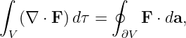
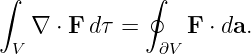
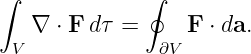
Two theorems provide the bridge:
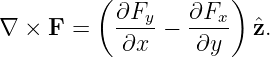
Equation (1) is the divergence theorem, also called Gauss’s theorem. Equation (2) is Stokes’
theorem. Both say that the accumulated interior behavior of a field is detected at a
boundary.
The purpose of this article is to derive these results rather than merely state them. We will then
apply them to all four Maxwell Equations, explore orientation conventions, and work through
examples directly connected to field measurements.
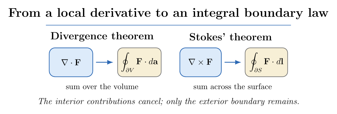
Figure 1. Two local-to-global bridges. Divergence accumulates over a volume to become flux
through its closed boundary. Curl accumulates across an oriented surface to become circulation
around its edge.
1 Before the theorems: the meaning of a boundary
A volume V has a closed surface boundary, written ∂V . The notation ∂V means the entire outer
boundary, not just one face.
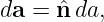
For a closed surface the area vector is defined by
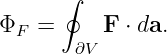
where n points outward from the volume. The flux is
The small circle on the integral sign reminds us the surface is closed.
A surface S need not be closed. It may have an edge, or boundary curve, ∂S. The line element dl
follows an orientation around that curve.
To specify an oriented surface, choose a unit Normal n. The positive traversal of ∂S is then
determined by the right-hand rule: curl the fingers of your right hand in the positive traversal
direction, and your thumb points along the chosen normal. Surface and boundary orientations
must agree.
2 Deriving the divergence theorem: one small box
Consider a rectangular box centered at (x,y,z) with side lengths Δx, Δy, and Δz. Its volume
is
Let
The outward normal on the right face is +x and on the left face is −x.
For a smooth field, the right-face flux to leading order in the dimensions is
The left-face flux is
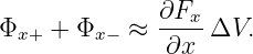
Add the two contributions:
| Φx+ + Φx− = |  Fx(x + Δx∕2) − Fx(x − Δx∕2) ![]](https://images.physicslibrary.org/cache/objects/1586/make4ht/GausssTheoremStokesTheoremAndIntegralFieldLaws9x.png) | |
|
| × ΔyΔz. | (9) |
The unshown y,z arguments in the brackets are held fixed.
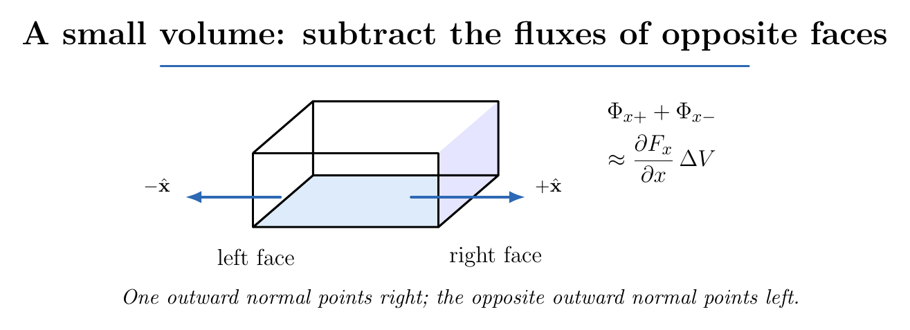
Figure 2. The two x faces have opposite outward normals. Their fluxes subtract, leaving the
change in Fx across the box. The other pairs of faces behave in the same way.
Expand each face value about the center:
| Fx(x + Δx∕2) | = Fx(x) +   + O(Δx2), | (10)
|
| Fx(x − Δx∕2) | = Fx(x) −  + O(Δx2). | (11) |
Subtracting, with a sufficiently smooth field, gives
Hence
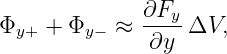
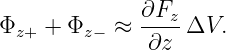
Repeat the argument for the other four faces:
The net flux through all six faces is therefore
| ΔΦF ≈ | 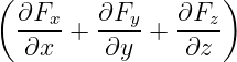 ΔV | (16)
|
| = | (∇⋅ F)ΔV. | (17) |
Dividing by ΔV and letting the box shrink recovers ED03’s local definition of divergence. The
important observation is that the spatial derivative is a difference between opposite boundary
fluxes.
3 From one box to an arbitrary finite volume
Now assemble many small cells into a finite volume V . Sum Equation (17) over all
cells:
Every face between two adjacent cells appears twice. The outward normal for cell 1 is the inward
normal for cell 2:
Since the field takes the same limiting value on both sides of a smooth interior face, the two flux
contributions cancel:
Only faces on the outer boundary survive. This is the essential reason the theorem
works.
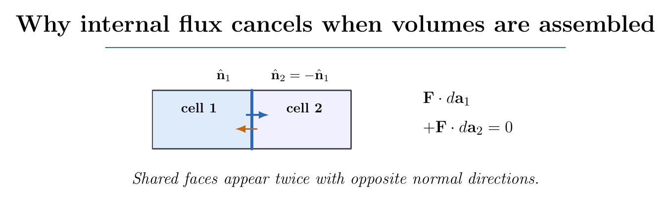
Figure 3. Subdividing a volume produces shared internal faces. Opposite outward normals make
the internal flux contributions cancel, leaving only the flux across the external boundary.
Refine the partition until the cells are arbitrarily small. The volume sum becomes a volume
integral and the surviving boundary flux becomes a surface integral:
This derivation assumes enough smoothness of F and sufficient regularity of the region and its
boundary to justify the limiting process. Piecewise smooth boundaries, such as those of a cube, are
included.
4 What Gauss’s theorem does and does not say
The left side is the total divergence accumulated throughout the volume. The right side is the net
outward flux. A region can contain positive and negative divergence that cancel in the total
integral.
Importantly, the theorem holds for a general sufficiently smooth vector field F. It does not require
spherical symmetry, a point charge, or even an electromagnetic interpretation.
Gauss’s theorem and Gauss’s law of electricity are different statements:
- Gauss’s theorem is a mathematical identity relating divergence and flux.
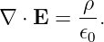
- Gauss’s electric law is a physical law specifying ∇⋅ E = ρ∕𝜖0.
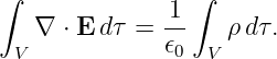
Their combination produces the electric flux law.
5 Worked example I: compute the flux two ways
Let
and take the rectangular region
Method A: integrate the divergence
Compute derivatives one at a time:
Thus
The volume integral becomes
| ∫
V ∇⋅ Fdτ | = ∫
0a ∫
0b ∫
0c(3x + 1) dz dy dx | (26)
|
| = bc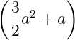 . | (27) |
Method B: add flux through six faces
At x = a, the outward normal is +x, so
At x = 0, Fx = 0, so Φx=0 = 0.
At y = b, the outward normal is +y and Fy = xb. Hence
At y = 0, the flux is zero. At z = c we have Fz = c, giving
while at z = 0 the flux is zero.
Therefore
| ∮
∂V F ⋅ da | = a2bc +  a2bc + abc | (31)
|
| = bc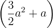 . | (32) |
This matches Equation (27) exactly.
6 Circulation and the meaning of an oriented loop
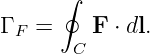
For a directed closed curve C, define the circulation of a vector field F as
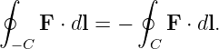
Circulation adds the components of the field along the path. Reversing the path reverses the
sign:
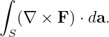
Similarly, reversing the chosen surface normal reverses the sign of
Both sides of Stokes’ theorem change sign together.
7 Deriving Stokes’ theorem: one small oriented loop
Start with a small rectangle in the xy plane, oriented counterclockwise as viewed from +z. Its sides
have lengths Δx and Δy. The positive normal is +z.
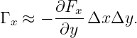
The horizontal bottom edge contributes approximately
while the horizontal top edge runs in the −x direction and contributes
The combined horizontal contribution is therefore
The right vertical edge runs along +y, and the left edge runs along −y:
| Γy ≈ | Fy(x + Δx∕2,y) Δy | |
|
| − Fy(x − Δx∕2,y) Δy | (39)
|
| ≈ |  ΔxΔy. | (40) |
Summing all four edges gives
| ΓF ≈ | 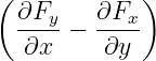 ΔxΔy | (41)
|
| = | (∇× F)z ΔA. | (42) |
The expression in parentheses is precisely the z component of curl derived in ED03. This is not a
coincidence: curl was constructed from the local circulation limit.
8 From a tiny loop to an entire surface
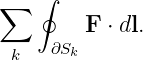
Divide an oriented surface S into many small oriented patches. Sum the circulation integrals
around their edges:
Every internal edge belongs to two neighboring patches. Compatible patch orientations traverse
their shared edge in opposite directions. Those two integrals cancel exactly, leaving only the outer
boundary ∂S.
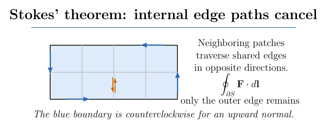
Figure 4. Compatible orientations around neighboring patches make each shared interior edge
cancel. When the small patches are added, only the outer boundary circulation remains.
For a sufficiently smooth field and surface, the local circulation of each tiny patch tends
to
In the limit the sum of all these patches becomes a surface integral:
This is Stokes’ theorem. The argument generalizes from small flat rectangles to sufficiently smooth
curved surfaces because each sufficiently small patch is locally planar.
9 Right-hand orientation, boundary direction, and holes
Stokes’ theorem demands a consistent pair of orientations:
- Choose a normal n over the surface.
- Use the right-hand rule to orient the boundary ∂S.
For a disk in the xy plane with normal +z, positive traversal is counterclockwise viewed from
above. For normal −z, the positive traversal is clockwise viewed from above.
A surface with a hole has an inner boundary as well as an outer boundary. Their compatible
orientations are opposite when viewed from the same side. The complete boundary ∂S includes
every boundary component.
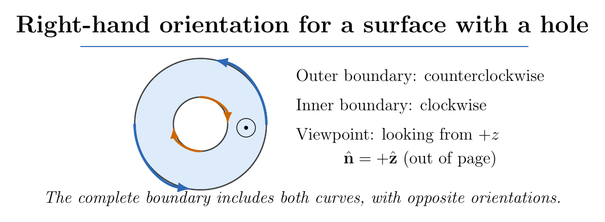
Figure 5. A surface normal determines its positive boundary orientation. For an annulus with
upward normal, the outer boundary runs counterclockwise and the inner boundary runs
clockwise, as viewed from above.
10 A powerful consequence: freedom to choose a spanning surface
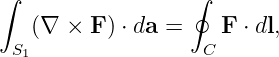
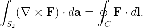
Suppose two smooth oriented surfaces S1 and S2 share the same boundary curve C with
compatible orientations. Applying Stokes’ theorem twice gives
Therefore
The equality requires that the field be sufficiently smooth on the surfaces and on the region where
the relevant theorem is applied. It cannot be used blindly across a field singularity. We will see why
later.
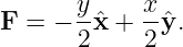
11 Worked example II: test Stokes’ theorem on a disk
Choose
Let C be the circle
traversed counterclockwise when viewed from +z.
Method A: line integral around the circle
Parameterize the boundary by
Then
The field on the circle is
Take the dot product:
| F ⋅ dl | =  (sin 2ϕ + cos 2ϕ) dϕ | (54)
|
| =  dϕ. | (55) |
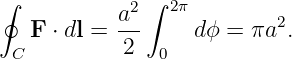
Therefore
Method B: surface integral of curl
Compute the curl:
But
Hence
On the planar disk da = zda, so
The methods agree.
What if the spanning surface is a hemisphere?
Choose the upper hemisphere with the same circular equatorial boundary, oriented so its outward
normal has nonnegative z component. The curl is still z. Its flux is the area of the hemisphere
projected onto the horizontal disk, which is πa2. The same boundary circulation is recovered
without integrating over a flat disk.
12 The four Maxwell equations: differential form
In vacuum using SI units, ED01 introduced
| ∇⋅ E | =  , | (61)
|
| ∇⋅ B | = 0, | (62)
|
| ∇× E | = − , | (63)
|
| ∇× B | = μ0J + μ0𝜖0 . | (64) |
The divergence theorem is applied to the first two laws. Stokes’ theorem is applied to the latter
two. Each conversion has an orientation convention, and the time derivatives must be interpreted
with the integration surface held fixed unless the motion of that surface is explicitly
included.
13 Derivation of Gauss’s electric law in integral form
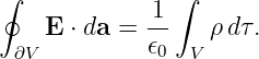
Start with the differential electric law:
Integrate both sides over a finite volume V :
Apply the divergence theorem to the left side:
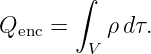
The total enclosed charge is
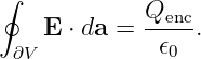
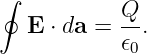
Therefore
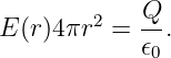
This is Gauss’s Law of electricity. Note the distinction between a law that specifies the divergence
and a theorem that converts divergence into boundary flux.
14 Worked example III: the electric field of a spherical charge distribution
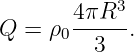
Take a stationary solid sphere of radius R carrying uniform volume charge density ρ0. Its total
charge is
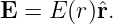
Spherical symmetry implies a radial field with magnitude depending only on radius:
Choose a concentric spherical Gaussian surface of radius r.
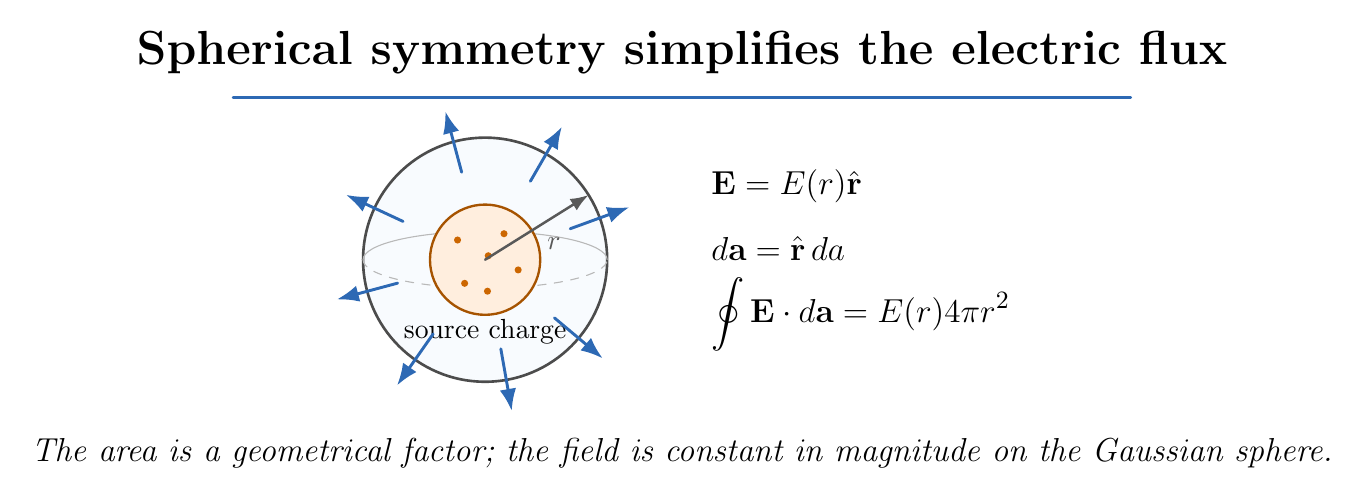
Figure 6. Spherical symmetry makes E normal to a concentric Gaussian sphere and equal in
magnitude everywhere on it. The flux integral becomes E(r)4πr2.
On the Gaussian sphere,
Because E(r) is constant on this spherical surface,
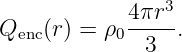
For 0 < r < R, the enclosed charge is only that inside radius r:
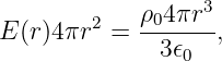
Gauss’s law gives
so
For r ≥ R, the Gaussian surface encloses all the charge:
Therefore
For positive charge density the field points outward; for negative density it points inward. At r = R
the two expressions agree.
Gauss’s law is always true, but extracting E(r) from the flux integral was easy here only because of
spherical symmetry.
15 Gauss’s law for magnetic fields
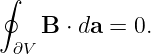
Apply the divergence theorem to
Integrating over V gives
The net magnetic flux through every closed surface is zero in classical Maxwell theory. Magnetic
field lines can cross a closed surface, but their signed inward and outward crossings sum to
zero.
This does not mean the magnetic field vanishes. A uniform nonzero magnetic field gives equal
inward and outward flux through opposite sides of a box, so the net closed-surface flux is
zero.
16 Worked example IV: magnetic circulation around a straight wire
Take an ideal infinitely long straight wire on the z axis carrying a steady current I along +z.
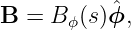
Rotational symmetry about the wire and translation symmetry along it imply a magnetic field of
the form
where s is cylindrical radius. The right-hand rule fixes the positive azimuthal direction for positive
I.
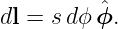
Choose a circular Amperian loop C of radius s centered on the wire. Traverse it counterclockwise
as viewed from +z. Along this loop,
Therefore
| ∮
CB ⋅ dl | = ∫
02πB
ϕ(s)sdϕ | (83)
|
| = 2πsBϕ(s). | (84) |
For steady current, the displacement-current contribution is zero. The integral Ampere law
gives
and hence
If I = 2.0 A and s = 0.010 m, then
This is 40 μT. The key step is not the integral itself; it is using symmetry to know the direction
and constant magnitude of B along the chosen loop.
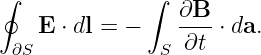
17 Faraday’s law from Stokes’ theorem
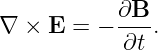
Start with
Integrate over an oriented fixed surface S:
Apply Stokes’ theorem on the left:
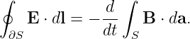
For a fixed surface, the time derivative can be moved outside the integral, giving
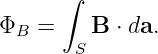
Define magnetic flux
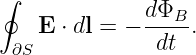
Then
The negative sign captures Lenz’s law through the right-hand orientation. The induced circulation
of E opposes the change in flux, not necessarily the flux itself.
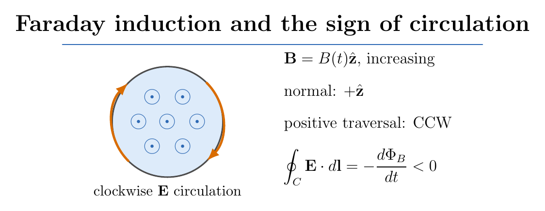
Figure 7. For an upward-increasing uniform magnetic field through a stationary loop, the induced
electric-field circulation is clockwise when viewed from above, corresponding to negative
circulation relative to the upward surface normal.
What changes when the conducting loop moves?
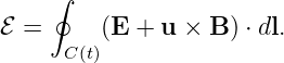
Equation (91) is the form derived for a fixed integration surface. For a moving material loop of
local wire velocity u, the relevant electromotive force in the nonrelativistic approximation
is
Under the usual conditions for a smooth moving loop, this equals minus the total time
derivative of the magnetic flux through the moving loop. The additional u × B term
is the motional contribution from the Lorentz force. ED37 treats the full distinction
carefully.
18 Worked example V: induced electric field around a changing flux
Suppose a uniform magnetic field fills a circular region and points along +z:
Choose a fixed circular loop of radius s entirely within that uniform-field region. By rotational
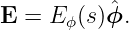
symmetry the induced electric field is azimuthal and has equal magnitude all around the
circle:
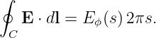
Using the counterclockwise positive orientation when viewed from above,
The flux is
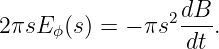
Faraday’s law gives
Therefore
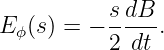
If s = 0.050 m and dB∕dt = +0.30 T∕s,
| Eϕ | = −0.0075 V∕m, | (101)
|
| ℰ | = −2.36 × 10⁻³ V. | (102) |
The sign indicates clockwise circulation relative to the chosen +z normal. A changing
magnetic field can create circulating electric field even in a region with no wire or free
charge.
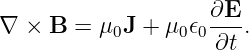
19 Ampere-Maxwell’s law from Stokes’ theorem
The differential equation is
Integrate over an oriented fixed surface S:
| ∫
S(∇× B) ⋅ da = | μ0 ∫
SJ ⋅ da | |
|
| + μ0𝜖0 ∫
S ⋅ da. | (104) |
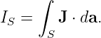
Apply Stokes’ theorem and define the conduction current through the surface as
For a fixed surface,
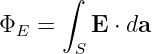
where
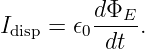
is electric flux. The second term is the displacement-current contribution:
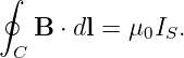
In magnetostatics, ∂E∕∂t = 0, and the familiar Ampere circuital law remains:
20 Why the displacement-current term is necessary
Consider a capacitor being charged by a current I(t). A circular Amperian loop surrounds the lead.
It can be spanned by different surfaces with the same boundary:
- A nearly flat surface cuts through the conducting lead and intercepts conduction
current.
- A bulging surface passes between the capacitor plates, where conduction current
through the vacuum gap is negligible.
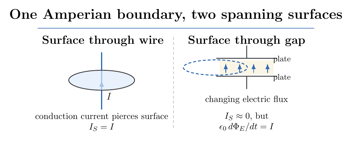
Figure 8. One boundary loop can be spanned by a surface cutting the wire or a curved surface
passing through the capacitor gap. The electric-flux time derivative across the gap supplies the
term that makes Ampere-Maxwell circulation independent of the chosen spanning surface.
In a simplified parallel-plate model, neglect edge fields and suppose the gap field is uniform. The
plate charge is
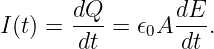
The current onto the plate is
Across a fixed gap surface of area A,
Thus the conduction current through one surface and the displacement current through the other
produce the same total circulation. The model is an illustrative quasistatic approximation; a real
charging capacitor may have fringing fields and radiative corrections.
21 The continuity equation as a Maxwell consistency condition
Take the divergence of the differential Ampere-Maxwell equation:
The divergence of a curl is zero:
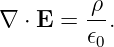
Use Gauss’s electric law,
Then
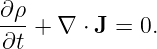
Dividing by μ0 gives charge conservation:
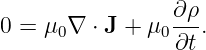
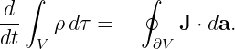
Integrating over a fixed volume and applying Gauss’s theorem gives its integral counterpart:
The charge inside a region decreases by exactly the outward current through its surface.
Without Maxwell’s displacement-current term, taking divergence of ∇×B = μ0J would incorrectly
force ∇⋅ J = 0 even when charge density is changing. The new term is required by local charge
conservation.
22 Integral laws can produce boundary jump conditions
The same theorems can be applied to a volume or loop made arbitrarily small across an interface
between two regions. This produces boundary conditions.
Let n point from region 1 to region 2. Suppose a surface charge density σ and surface current
density K may exist at the interface.
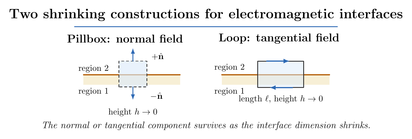
Figure 9. A thin Gaussian pillbox isolates normal field components across an interface; a
shrinking rectangular Stokes loop isolates tangential components. These two limits lead to the
electromagnetic jump conditions.
Electric normal component: thin pillbox
Take a short cylinder of face area A straddling the interface. The top outward normal is +n and
bottom outward normal is −n.
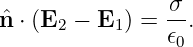
As its height tends to zero, flux through its sidewall vanishes for bounded fields. Gauss’s electric
law becomes
Cancel A:
Magnetic normal component
Apply the same pillbox to ∮
B ⋅ da = 0:
The normal component of B is continuous across the interface in Maxwell theory.
Electric tangential component: small loop
Let a rectangular loop of length ℓ run along a tangent direction t, with short sides crossing the
interface. As its height tends to zero, the flux time derivative is negligible for bounded, nonsingular
∂tB.
Faraday’s law gives
Because t is any tangent direction,
Magnetic tangential component: surface current
The same shrinking loop applied to Ampere-Maxwell’s law encloses a surface current K. Under
ordinary finite-field conditions, the displacement-flux contribution vanishes in the shrinking-height
limit. The result is
These four conditions are the vacuum microscopic field jump conditions. In matter they can be
rewritten using D and H to distinguish free and bound sources, a topic developed later in the ED
sequence.
23 Where the smooth-field proofs need care: singular sources
The divergence theorem was derived for a smooth field in the region of integration. A point-charge
field is singular at the charge location:
For r > 0,
But the flux through a sphere of any radius enclosing the origin is
There is no contradiction: the classical smooth-field hypotheses fail at r = 0. If the origin is
removed from the integration region, an inner boundary appears and its flux accounts for the
missing contribution.
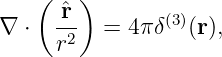
The compact distributional identity is
where δ(3) is a three-dimensional Dirac delta distribution. ED05 will derive this carefully and
examine line and surface singular sources.
Similarly, consider a circulating field F = ϕ∕s in a region excluding the z axis. Away from the axis,
its ordinary curl is zero, yet a circle surrounding the axis has nonzero circulation. A
disk spanning that circle passes through a singularity, so the ordinary smooth Stokes
theorem cannot be applied over that disk without accounting for the excluded core.
The same issue can be understood by choosing a punctured surface that has an inner
boundary.
The lesson is general: when an apparent integral/differential contradiction occurs, check whether
the field or domain violates the regularity assumptions.
24 How to decide which integral law is useful
The four integral Maxwell equations have complementary geometric forms:
- Electric Gauss law: charge enclosed by a closed surface controls net electric flux.
- Magnetic Gauss law: net magnetic flux through any closed surface is zero.
- Faraday law: changing magnetic flux through an oriented surface controls electric
circulation along its boundary.
- Ampere-Maxwell law: conduction current and changing electric flux through an
oriented surface control magnetic circulation along its boundary.
A closed surface suggests a divergence/Gauss problem. A closed curve suggests a curl/Stokes
problem. But symmetry determines whether the resulting integral can be used to solve directly for
the field magnitude.
25 Laboratory interpretation: what would we measure?
EDL potential maps estimate electric potential at a collection of positions. In an electrostatic
regime, neighboring measurements can approximate the gradient, and a numerical surface integral
can estimate electric flux through an imagined Gaussian surface. The field reconstructed this way
inherits sensor placement, calibration, interpolation, and boundary-error uncertainties.
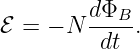
A small magnetic pickup coil responds to changing magnetic flux. For N identical tightly coupled
turns, the induced open-circuit emf under ordinary conditions is approximately
The coil does not measure B at one exact point; it responds to an area integral of B, followed by a
time derivative.
A Hall sensor, by contrast, reports a calibrated component of the local field. Mapping B around
a wire and then numerically evaluating ∮
CB ⋅ dl is an instructive experimental test
of the magnetostatic circulation law, subject to sensor alignment and limited spatial
resolution.
These distinctions connect the mathematical operations with what physical probes actually
measure.
26 A local-to-global comparison
The two theorems can be remembered from how subdivisions cancel:
- Volume cells share a face. Their outward face normals are opposite, so internal face
flux cancels.
- Surface patches share an edge. Their positive edge traversals are opposite, so internal
edge circulation cancels.
Thus a boundary of a boundary does not contribute: the surviving integral lives only on the actual
outer boundary. The deeper mathematics of this pattern appears in more advanced
treatments of differential forms, but the small-cell construction already captures the essential
physics.
27 Common errors and diagnostic checks
- Confusing Gauss’s mathematical theorem with Gauss’s physical electric law.
- Forgetting that the normal on a closed surface points outward.
- Taking the line integral of E around a curve but choosing a surface normal inconsistent
with the curve direction.
- Assuming all nonzero local divergence or curl produces a nonzero integral over every
region; cancellations can occur.
- Trying to solve for E or B from an integral law without using the necessary source
symmetry.
- Replacing a partial time derivative by a total flux derivative for a moving loop without
accounting for motional emf.
- Dropping the displacement-current term from Ampere’s law during charging or other
time-dependent processes.
- Applying Stokes’ theorem across a singularity without excluding the singular set or
treating it distributionally.
- Ignoring inner boundaries of multiply connected surfaces.
- Interpreting a vanishing net magnetic flux through a closed surface as evidence that B
must vanish everywhere.
28 Practice problems
- For F = (x, 2y, 3z), compute the flux through the closed unit cube by both surface
integration and the divergence theorem.
- For F = (yz,xz,xy), compute ∇⋅ F and the net flux through any closed cube.
- Compute the circulation of F = (−y,x, 0) around a counterclockwise circle of radius a
in the xy plane; verify with Stokes’ theorem.
- Repeat Problem 3 with the boundary traversed clockwise. Explain both sign changes.
- Explain how a flat disk and an upper hemisphere with the same oriented boundary
can yield equal curl fluxes.
- A point charge Q lies outside a closed Gaussian surface. What is its net electric flux
through that surface? Does it necessarily produce zero electric field on the surface?
- For a uniform B = B0z, compute the net flux through a closed cube and explain the
result using face normals.
- For a stationary circular loop of radius a with uniform B(t) through its interior, derive
the induced circulation and identify the sign for increasing +z flux.
- In a charging ideal parallel-plate capacitor, explain why Ampere’s original
conduction-current term is insufficient when the spanning surface passes between the
plates.
- Derive the normal-electric-field jump condition using a pillbox containing surface
charge σ.
- Explain the difference between the ordinary divergence of r∕r2 for r > 0 and its
distributional divergence on all of ℝ3.
- Derive the integral charge-conservation law from the local continuity equation and the
divergence theorem.
29 Summary and bridge to ED05
Gauss’s theorem is built from opposite fluxes through tiny volume faces. When many cells are
assembled, internal face contributions cancel:
Stokes’ theorem is built from oriented circulation around tiny surface patches. When the patches
are assembled, internal edge contributions cancel:
Using Maxwell’s differential laws, these become the four integral electromagnetic laws:
| ∮
∂V E ⋅ da | =  , | (132)
|
| ∮
∂V B ⋅ da | = 0, | (133)
|
| ∮
∂SE ⋅ dl | = − , | (134)
|
| ∮
∂SB ⋅ dl | = μ0IS + μ0𝜖0 . | (135) |
The last two equations assume fixed integration surfaces as written.
ED05 will revisit these identities when charge and current are concentrated at points, lines, or
surfaces. There, delta distributions provide a rigorous bridge between singular sources and their
integral effects.
References
References
[1] D. J. Griffiths, Introduction to Electrodynamics, 5th ed., Cambridge University Press,
2023.
[2] E. M. Purcell and D. J. Morin, Electricity and Magnetism, 3rd ed., Cambridge
University Press, 2013.
[3] H. M. Schey, Div, Grad, Curl, and All That, 4th ed., W. W. Norton, 2005.
[4] M. L. Boas, Mathematical Methods in the Physical Sciences, 3rd ed., Wiley, 2006.
[5] A. Zangwill, Modern Electrodynamics, Cambridge University Press, 2013.