Electric Current and Conservation of Charge

(Topic)

E02: Electric Current and Conservation of Charge

Foundations of Electricity and Electrical Measurement, mini-lecture 2.

In E01, we introduced electric charge and potential difference. A battery can maintain a potential difference between two terminals, and a voltmeter measures the potential difference between two selected points. What changes when a conducting path connects the terminals through an electrical load?

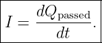
Charges begin to move in response to the electrical environment. Their motion produces an electric current. This lecture develops current from the transport of charge, connects current to the microscopic motion of carriers, and derives the circuit junction rule from conservation of charge.

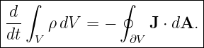
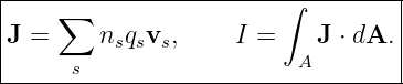
The first equation is

|-------------| | dQpassed | I = -------. | -------dt------

(1)

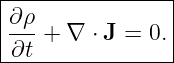
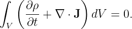
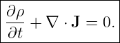
The deeper equation, which applies locally in continuous media, is

|∂ρ--------------| |---+ ∇ ⋅ J = 0.| -∂t--------------|

(2)

The second equation says that charge cannot disappear from a region without leaving through its boundary. In ordinary circuit analysis, that simple physical statement becomes Kirchhoff’s current law.

Learning objectives

After this lesson, the reader should be able to:

define current as signed charge flow through an oriented surface;
convert among current, elapsed time, transferred charge, and number of charge carriers;
explain conventional current and why electrons drift in the opposite direction in a metal;
derive the drift-current relationship from a swept volume;
express current as the flux of current density through a surface;
derive the charge balance for a circuit junction and state the conditions for the usual Kirchhoff current law;
derive the integral and differential forms of charge continuity;
connect these ideas to safe ammeter and voltmeter connections in EDL01.

1 What is electric current?

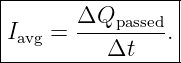
Imagine selecting a cross section of a conductor and choosing a direction Normal to its surface. We keep track of the signed charge that crosses this surface in that direction. If a net amount ΔQ_passed crosses during the time interval Δt, the average current is

|----------------| | ΔQpassed | |Iavg = ---------.| ----------Δt------

(3)

The direction convention matters. A positive charge moving along the selected normal contributes positive current; a negative charge moving in the opposite direction also contributes positive current.

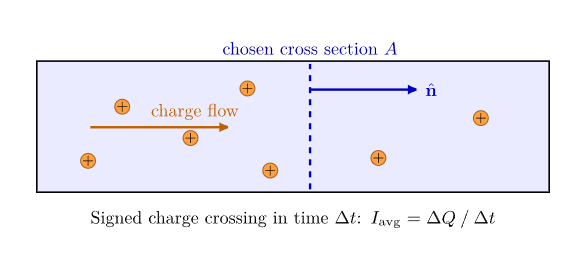
Figure 1. Electric current measures signed charge passing through a chosen cross section per unit time. The normal vector establishes the positive direction.

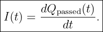
For an interval that is made arbitrarily short, this gives the instantaneous current:

|------------------| | dQpassed(t) | |I(t) = ----------.| ------------dt------

(4)

Here Q_passed(t) is a cumulative, signed transported charge through the selected surface, not necessarily the total charge stored in a wire or capacitor.

The SI unit of current is the ampere, symbol A:

1 A = 1 C∕s.

(5)

The elementary charge has the exact SI value

e = 1.602176 634 × 10− 19 C.

(6)

Consequently, a current of 1 A corresponds in magnitude to the transport of about 6.24 × 10¹⁸ elementary charges through a cross section each second. The SI ampere is defined through the fixed numerical value of e, not through a mechanical force between wires.

1.1 Example: charge carried in a short time

A steady current of 3.0 mA flows for 2.0 min. The magnitude of transported charge is

\|ΔQ\|	= \|I\|Δt	(7)
	= (3.0 × 10⁻³ A)(120 s)	(8)
	= 0.36 C.	(9)

The corresponding count of elementary charges is

0.36 18 N = 1.602-176-634-×-10−-19-≈ 2.25 × 10 .

(10)

This count represents charge crossings, not the number of new electrons created by the source.

2 Conventional current and moving charge carriers

Conventional current is defined in the direction in which positive charge would move. This definition applies even if the actual mobile carriers are negatively charged electrons.

In a metal, the positive ions that form the lattice are approximately stationary. The mobile carriers are electrons. If the conventional current is rightward, the mean electron drift is leftward.

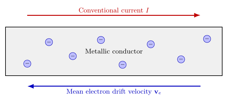
Figure 2. In a metallic wire, electron drift and conventional current point in opposite directions. Random microscopic motion is superposed on the small average drift.

The definition is more general than metallic conduction. In an electrolyte, positive and negative ions can move in opposite directions, while both kinds of carrier contribute to a conventional current in the same direction.

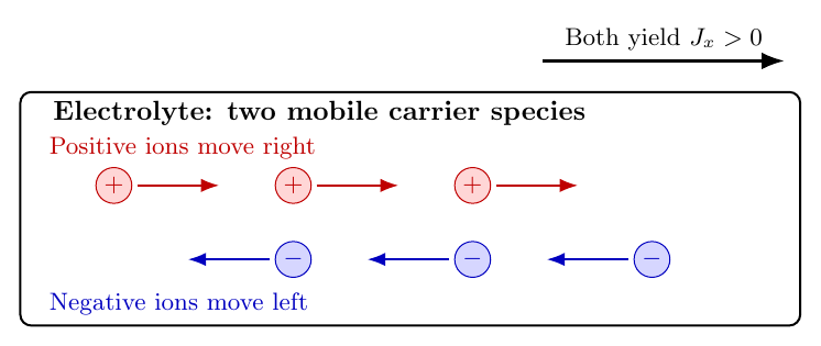
Figure 3. Positive ions moving right and negative ions moving left both contribute positive rightward current.

The direction of current is therefore a sign convention for charge transport, not a claim about which particular particles must move.

3 Time-dependent current and the transported-charge graph

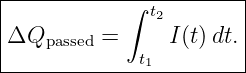
If the current is not constant, the transported charge is found by integration:

|----------------------| | ∫ t2 | |ΔQpassed = I(t)dt.| -------------t1---------

(11)

The graph of Q_passed(t) has slope I(t). A large positive slope means a large positive current. A negative slope means that the net signed charge transport is in the opposite direction.

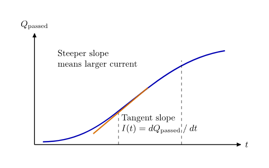
Figure 4. The local slope of cumulative transported charge versus time equals instantaneous current. The signed area beneath a current-versus-time curve gives transported charge.

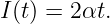
As a simple model, suppose

Qpassed(t) = αt2,

(12)

where α has units of C∕s². Differentiation gives

I(t) = 2αt.

(13)

A constant current corresponds to a straight-line Q_passed graph. An alternating current need not transport a nonzero net charge over an entire cycle, even though charges move throughout the cycle.

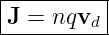
4 Why moving charges produce current: the drift model

Consider identical mobile carriers with number density n (carriers per unit volume), charge q per carrier, and average drift velocity v_d. Let A be an area perpendicular to their motion and let v_d be the signed velocity component along the chosen normal.

During a short interval Δt, carriers within a length v_dΔt cross the surface, with the sign interpreted algebraically. The swept volume is A|v_d|Δt, and the magnitude of the crossing count is

N = nA |vd|Δt.

(14)

For signed transport,

ΔQpassed = nqAvd Δt.

(15)

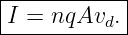
Dividing by Δt gives the drift-current relation:

|-----------| I = nqAvd. | -------------

(16)

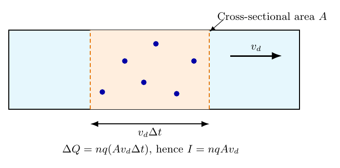
Figure 5. The carriers inside a swept volume Av_dΔt cross a conductor section during Δt. The direction of v_d is signed.

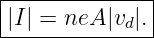
For electrons, q = −e. If their signed drift velocity is negative, the resulting conventional current is positive. When only magnitudes are used, we can write

|--------------| ||I| = neA |vd|. ---------------

(17)

4.1 Why the drift speed is usually slow

A metallic wire contains an enormous density of mobile electrons. Even a small average directed velocity can therefore transport a substantial amount of charge per second. An illustrative conduction-electron density for copper is n ≈ 8.5 × 10²⁸ m⁻³, using one effective conduction electron per atom.

For a 1.0 mm diameter wire carrying 2.0 A,

A = π (0.50 × 10− 3)2 ≈ 7.85 × 10− 7 m2.

(18)

The magnitude of mean electron drift speed is

\|v_d\|	=	(19)
	≈ 1.87 × 10⁻⁴ m∕s	(20)
	= 0.187 mm∕s.	(21)

The result is an average drift speed, not the speed of random microscopic motion or the propagation speed of an electromagnetic signal along a circuit. A circuit can respond much more quickly than any individual electron can travel around it.

5 From current to current density

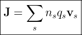
Current is a scalar with a chosen signed reference direction. To describe charge flow throughout a continuous medium, we introduce the vector current density J:

|----------| -J-=-nqvd--|

(22)

for a single mobile species, or more generally

|----∑---------| J = nsqsvs| | s | ----------------

(23)

for several species. Its SI unit is A∕m².

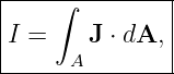
Through an oriented surface A, the total current is

|----∫---------| | | |I = J ⋅ dA,| ------A---------

(24)

where dA = ndA. The dot product selects the component of current density normal to the surface.

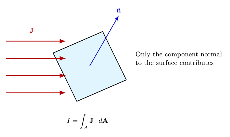
Figure 6. The flux of current density through an oriented surface determines its signed current. Flow parallel to the surface contributes no crossing.

If J is uniform and perpendicular to a flat cross section,

I = JA.

(25)

A wire does not need uniform J for the integral formula to hold. In later lectures, resistance and conductivity will explain how an Electric Field influences J in specific materials.

6 Conservation of charge at a circuit junction

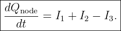
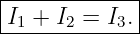
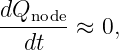
Imagine an electrically small junction where currents I₁ and I₂ enter and current I₃ leaves. Suppose the total charge stored in the junction region is Q_node(t).

Over a short time dt, the entering charge is (I₁ + I₂)dt and the leaving charge is I₃dt. Conservation of charge requires

dQnode = (I1 + I2 − I3)dt.

(26)

Therefore,

|----------------------| |dQnode- | | dt = I1 + I2 − I3. ------------------------

(27)

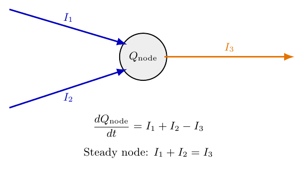
Figure 7. Current imbalance changes the amount of charge stored in the junction region. If the node charge is approximately constant, the inflow equals the outflow.

If the node has negligible net charge accumulation,

dQnode -------≈ 0, dt

(28)

then

|I-+-I--=-I-.| --1---2----3--

(29)

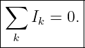
This is Kirchhoff’s current law (KCL), also called the junction rule. With all branch currents given algebraic signs according to an agreed convention, the rule is commonly written

∑----------| | Ik = 0.| | k | ------------

(30)

The equation expresses charge conservation at a circuit node. It is not an independent assumption about how charges behave.

6.1 What if charge accumulates?

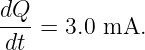
If 5.0 mA enters a small isolated region while 2.0 mA leaves, the stored charge increases at

dQ --- = 3.0 mA. dt

(31)

The simplified equal-inflow/equal-outflow statement cannot be applied to the same region without accounting for accumulation. In an ordinary lumped circuit, charge storage is modeled explicitly, often with a capacitor.

7 Charge conservation in a continuous medium

A circuit node is a special case of a more general three-dimensional statement. Choose any fixed volume V bounded by a closed surface ∂V . Let ρ(r,t) be electric charge density.

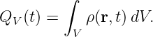
The total charge in the volume is

∫ Q (t) = ρ(r,t)dV. V V

(32)

Current leaving the closed surface is positive when measured with the outward surface normal. Consequently,

|--∫------------∮----------| |d- ρ dV = − J ⋅ dA.| -dt--V-----------∂V---------

(33)

This is the integral continuity equation.

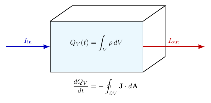
Figure 8. Charge in a fixed control volume decreases when the outward current flux exceeds the inward current flux.

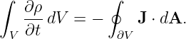
For a fixed volume, the time derivative can be brought inside the volume integral:

∫ ∮ ∂-ρdV = − J ⋅ dA. V ∂t ∂V

(34)

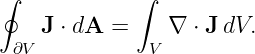
The divergence theorem states that

∮ ∫ J ⋅ dA = ∇ ⋅ J dV. ∂V V

(35)

Thus

∫ ( ) ∂ρ- V ∂t + ∇ ⋅ J dV = 0.

(36)

Because this holds for every suitably chosen volume, the integrand must vanish at each regular point:

|----------------| |∂ρ-+ ∇ ⋅ J = 0.| -∂t--------------|

(37)

This is the differential continuity equation. When ∇⋅ J > 0, more charge flows outward than inward locally, so ∂ρ∕∂t < 0.

For steady charge distributions,

∂ρ ---= 0 = ⇒ ∇ ⋅ J = 0. ∂t

(38)

Steady current may be present even when there is no local charge accumulation. This is the continuum counterpart of the ordinary KCL.

7.1 Preview of Maxwell’s equations

Charge conservation remains valid for time-dependent electromagnetic fields. In Maxwell’s theory, the conduction current is complemented by the displacement-current term when describing the magnetic field produced by a charging capacitor. This is why a circuit can have a meaningful total current across a capacitor’s dielectric even when no electrons cross that dielectric. The full field-theory derivation belongs in later EM articles.

8 Direct current and alternating current

In a steady direct-current (DC) circuit, branch currents are constant in time, after transients have subsided:

I(t) = I . 0

(39)

For a sinusoidal alternating current (AC), a simple mathematical model is

I(t) = I cos(ωt + ϕ), 0

(40)

where ω is angular frequency and ϕ is phase. The signed current reverses direction during each cycle. Over a complete cycle, its integral can be zero even though charge moves continuously.

Understanding frequency, phase, and RMS values is reserved for E16. For now, we only need to recognize that the instantaneous current is a signed rate, not simply a count of particles moving in one fixed direction.

9 Current in an electrical laboratory

A voltmeter compares potentials at two points; an ammeter measures current through a branch. For ordinary low-frequency circuit measurements, the connections are different:

A voltmeter is connected across the element of interest, in parallel. An ideal voltmeter has infinite input resistance.
An ammeter is inserted into the path carrying the current, in series. An ideal ammeter has zero series resistance.

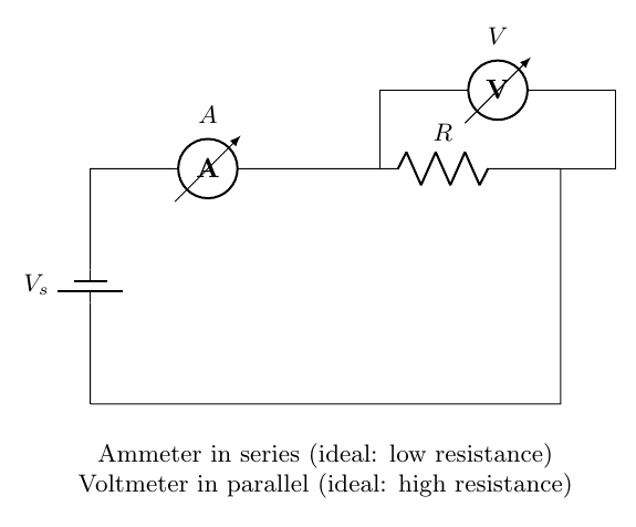
Figure 9. A current meter belongs in series with a branch; a voltmeter belongs across the element being measured. Real meters are not ideal and can change the circuit.

For example, an ideal 6.0 V source and a 1.2 kΩ resistor produce, in the simple resistance model,

6.0 V I = ------------= 5.0 mA. 1.2 × 103 Ω

(41)

This relation uses Ohm’s law, which E03 will develop carefully. In EDL01, the measurement is performed with real sources, meter leads, and a measured resistor value rather than the ideal values used here.

Low-voltage measurement safety

Use only a low-voltage, current-limited DC source for introductory measurements. De-energize the circuit before moving the meter leads between voltage and current jacks. Use the correct meter input, fuse rating, and current range. Never connect a meter configured for current measurement straight across a battery or supply; its low internal resistance can create a near-short circuit. Never use these procedures on mains wiring.

10 Current, power, and the speed of electrical response

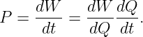
If charge dQ crosses a potential difference V in time dt, the associated rate of electrical energy transfer in a lumped element is

dW dW dQ P = dt--= dQ--dt-.

(42)

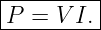
Using dW∕dQ = V for the adopted passive-sign convention gives

|--------| P--=-V-I.-

(43)

This relation will be developed with circuit elements and sign conventions in E04. Current indicates the rate of charge transport, not by itself the rate of energy transfer. A potential difference is also involved.

The small drift speed estimated earlier does not mean an electrical device must wait for one electron to travel from a distant source to the load. Mobile charges already exist throughout a connected conductor. Electrical and electromagnetic disturbances propagate through the circuit and the surrounding fields, while individual electrons typically drift much more slowly.

11 Common misconceptions

Current is not the amount of charge stored; it is the time rate of signed charge crossing a selected surface.
Conventional current does not necessarily coincide with the motion of the physical charge carriers.
Electrons are not the only possible carriers. Ions and holes can also contribute to current.
Slow electron drift does not imply equally slow propagation of an electrical signal.
Charge cannot be consumed by a resistor, although electrical energy can be converted into thermal energy.
Equal currents entering and leaving a junction follow when the junction stores negligible changing net charge.
Zero time-averaged AC current does not imply that no charge moves.
An ammeter is not connected like a voltmeter.

12 Summary and bridge to E03

|----------------------------∫---------| I = dQpassed-, ΔQ = I(t)dt.| | dt passed | ----------------------------------------

(44)

|------------------------∫---------| | ∑ | |J = nsqsvs, I = J ⋅ dA.| ------s-------------------A--------|

(45)

|---------∮-------------------------------| dQV-- ∂ρ- | | dt = − J ⋅ dA, ∂t + ∇ ⋅ J = 0.| -----------∂V------------------------------

(46)

The first two relationships quantify moving charge. The last two express charge conservation in a finite region and at a point. For an ordinary lumped-circuit node with negligible charge accumulation, they reduce to Kirchhoff’s current law. E03 will address the next question: what controls the amount of current that flows for a given electrical excitation?

References

[1] OpenStax, University Physics, Volume 2, Sections 9.1 and 9.2, “Electrical Current” and “Model of Conduction in Metals.”

[2] OpenStax, University Physics, Volume 2, Section 10.3, “Kirchhoff’s Rules.”

[3] National Institute of Standards and Technology, Definitions of SI Base Units, section on the ampere.

[4] D. J. Griffiths, Introduction to Electrodynamics, sections on electric current and conservation laws.

"Electric Current and Conservation of Charge" is owned by bloftin.
(view preamble)