Continuous Strings, Standing Waves, and Normal Modes
A long chain of coupled oscillators approaches a continuous medium when the lattice spacing
becomes small compared with the wavelength.
The simplest continuous wave-bearing mechanical system is a stretched string.
Let
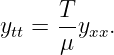
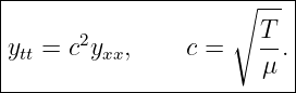
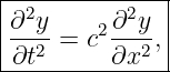
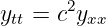
For small slopes, the transverse motion obeys
where
This is the one-dimensional wave equation.
A string of length
fixed at both ends cannot support arbitrary single-frequency shapes.
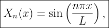
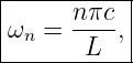
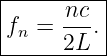
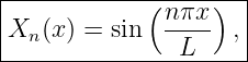
The boundary conditions select a discrete family of normal modes:
with
Thus a continuous system has infinitely many normal modes.
The finite-dimensional modal ideas from M06-04 and M06-05 become a Fourier-series description of
a continuous displacement field.
1 Small transverse displacement model
Consider a string whose equilibrium position lies along the
axis.
Let
be its transverse displacement.
Assume:
- the displacement is small,
- the slope satisfies |∂y∕∂x|≪ 1,
- the tension magnitude is nearly constant,
- longitudinal motion is neglected,
- the string is perfectly flexible.
These assumptions produce the linear string model.
2 Force balance on a small element
Take an element extending from
to
Its mass is
The tension at each end is tangent to the string.
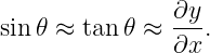
Let the local tangent angle be
For small slope,
The net transverse force is therefore
| dFy | = T![[ ∂y || ∂y || ]
---|| − ---||
∂x x+dx ∂x x](https://images.physicslibrary.org/cache/objects/1502/make4ht/ContinuousStringsStandingWavesAndNormalModes12x.png) | (13)
|
| ≈ T dx. dx. | (14) |
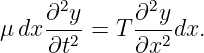
Newton’s second law gives
Canceling
gives
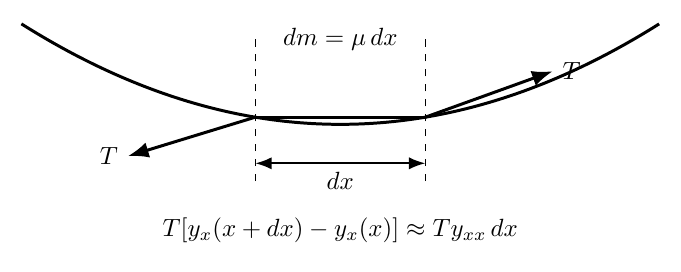
Figure 1. A small string element experiences tension forces tangent to the string at its two ends.
For small slopes, the difference of their transverse components is proportional to the local
curvature.
3 Wave speed
Divide by
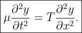
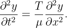
Then
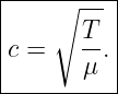
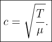
Define
Thus
The dimensions are
Larger tension increases the wave speed.
Larger linear mass density decreases it.
4 Traveling-wave solutions
A function of the form
satisfies the wave equation.
It represents a shape traveling to the right at speed
Similarly,
travels to the left.
The general d’Alembert solution on an unbounded string is
Standing Waves arise when oppositely traveling waves of the same frequency interfere.
5 A sinusoidal traveling wave
Consider
Substitution into the wave equation gives
Therefore
for positive
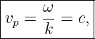
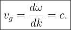
The ideal string is nondispersive:
and
Unlike the discrete chain of M06-06, the ideal continuous string has a linear dispersion
relation.
6 Standing wave from two traveling waves
Take equal-amplitude waves traveling in opposite directions:
and
Their sum is
Using a trigonometric identity,
The spatial shape
does not translate.
Its amplitude oscillates in time.
This is a standing wave.
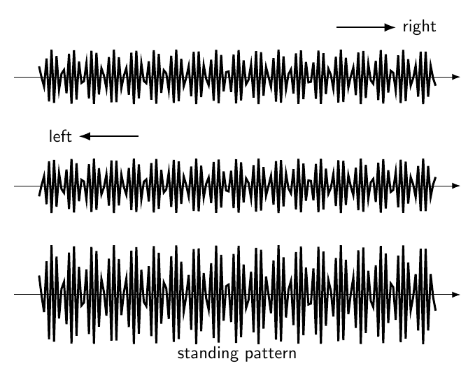
Figure 2. Two equal-frequency waves traveling in opposite directions can combine into a standing
wave. The standing-wave nodes remain fixed in space while the displacement between them
oscillates.
7 Fixed-end boundary conditions
Now consider a string extending from
to
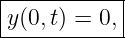
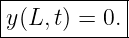
If both ends are fixed,
and
These boundary conditions select the allowed standing-wave patterns.
8 Separation of variables
Seek a product solution
Substitution into
gives
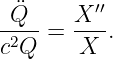
Divide by
The left side depends only on time.
The right side depends only on position.
Therefore both must equal a constant.
For oscillatory normal modes, write that constant as
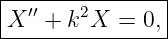
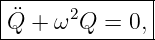
Then
and
where
9 Solving the spatial equation
The spatial solution is
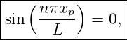
The boundary condition
requires
Thus
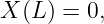
The second boundary condition,
requires
Therefore
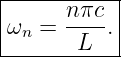
10 Normal frequencies
Since
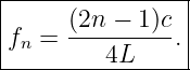
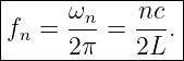
The ordinary frequencies are
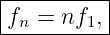
Therefore
with
The fixed-fixed ideal string has an exact harmonic spectrum.
11 Normal-mode shapes
Ignoring an arbitrary normalization constant,
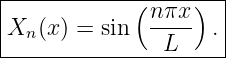
The first few modes are:
| X1(x) | = sin  , , | (64)
|
| X2(x) | = sin  , , | (65)
|
| X3(x) | = sin  . . | (66) |
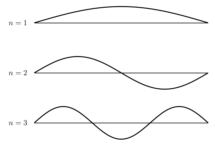
Figure 3. The first three fixed-fixed string modes. Increasing mode number adds internal nodes
and shortens the wavelength while preserving zero displacement at both endpoints.
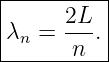
12 Allowed wavelengths
For
and
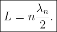
Thus the string length contains
half-wavelengths:
13 Nodes and antinodes
A node is a point whose displacement remains zero throughout the normal-mode motion.
For mode
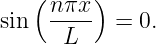
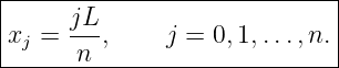
nodes satisfy
Therefore
The endpoints are always nodes.
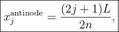
Antinodes occur where the magnitude of the sine is one:
for the appropriate integer values of
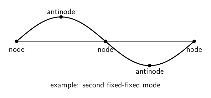
Figure 4. Nodes are fixed zeros of a standing-wave mode. Antinodes lie halfway between adjacent
nodes and undergo the largest displacement magnitude.
14 Mode orthogonality
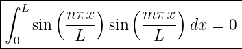
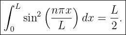
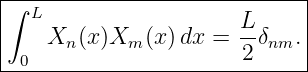
The fixed-end mode functions satisfy
for
For
Combining both cases,
This is the continuum analogue of eigenvector orthogonality.

Figure 5. String normal modes act like orthogonal basis vectors in a function space. An arbitrary
displacement shape can be projected onto them to obtain its modal amplitudes.
15 General modal expansion
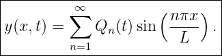
Because the modes form a complete basis for suitable fixed-end shapes,
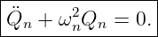
Substituting into the wave equation gives, mode by mode,
Thus
Therefore
| y(x,t) | = ∑
n=1∞![[An cos ωnt + Bn sin ωnt]](https://images.physicslibrary.org/cache/objects/1502/make4ht/ContinuousStringsStandingWavesAndNormalModes84x.png) | (85)
|
| × sin  . . | (86) |
A continuous string is therefore an infinite collection of independent harmonic normal
coordinates.
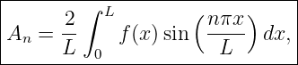
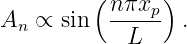
16 Initial displacement determines An
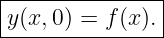
Suppose
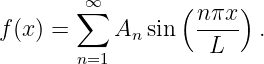
At
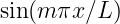
Multiply by
and integrate.
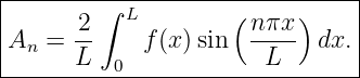
Orthogonality gives
These are Fourier sine coefficients.
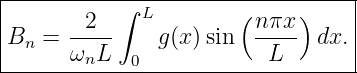
17 Initial velocity determines Bn
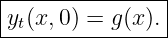
Suppose
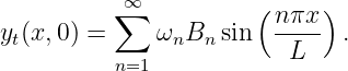
Differentiate the modal expansion:
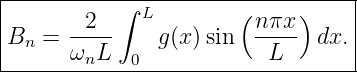
Project using orthogonality:
The complete initial state
therefore determines every modal coordinate.
This is the continuous-field analogue of projecting finite-dimensional initial position and velocity
onto Normal eigenvectors.
18 Example 1: fundamental frequency of a string
Let
| L | = 0.650 m, | (96)
|
| T | = 120 N, | (97)
|
| μ | = 5.00 × 10⁻³ kg∕m. | (98) |
The wave speed is
| c | = 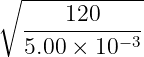 | (99)
|
| =  | (100)
|
| ≈ 154.9 m∕s. | (101) |
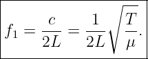
The fundamental frequency is
| f1 | =  | (102)
|
| =  | (103)
|
| ≈ 119.2 Hz. | (104) |
The next two harmonics are
19 Example 2: string plucked into a triangular shape
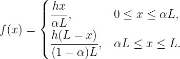
Suppose the string is displaced to height
at
with
and is otherwise straight between the endpoints and the pluck point.
Thus
Assume the string is released from rest:
Therefore
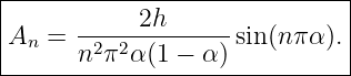
Evaluating the Fourier integral gives
The motion is
| y(x,t) | = ∑
n=1∞A
n cos(ωnt) | (113)
|
| × sin  . . | (114) |
The pluck position controls which harmonics are excited.

Figure 6. A triangular pluck is not a single normal mode. It is decomposed into an infinite Fourier
sine series. The pluck position determines the relative amplitudes of the harmonics.
20 Midpoint pluck
For a midpoint pluck,
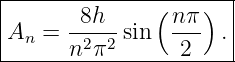
Then
For even
Therefore
Only odd harmonics are excited by a perfectly symmetric midpoint pluck.
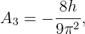
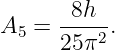
For the first few nonzero terms,
and
The
decay reflects the relatively smooth, piecewise-linear initial shape.
21 Nodes suppress selected modes
Suppose the string is plucked at a position
A mode whose node lies exactly at
can have zero overlap with certain symmetric pluck profiles.
For the triangular result,
Thus if
that harmonic is absent.
The geometry of the initial condition therefore selects the modal spectrum.
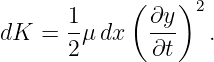
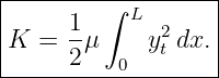
22 Kinetic energy of a string
The kinetic energy of an element
is
Thus
23 Elastic potential energy
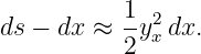
For small slope, the extra length of a string element is approximately
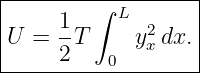
Work against the tension gives
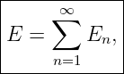
Therefore total energy is
24 Energy in modal coordinates
Insert
Orthogonality eliminates cross terms.
The result is
where
Thus each string normal mode behaves as an independent harmonic oscillator.
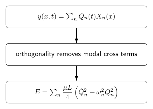
Figure 7. Orthogonality diagonalizes the string energy. Each modal coordinate Qn(t) carries its
own conserved harmonic-oscillator energy in the ideal string model.
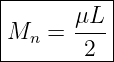
25 Effective modal mass
The modal energy can be written
Comparing with the previous expression gives
for the unnormalized choice
The numerical modal mass depends on the normalization convention for
The physical field
does not.
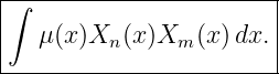
26 Continuum orthogonality as mass orthogonality
For a nonuniform string with position-dependent density
the natural modal inner product contains a Weight:
This is the continuous analogue of the finite-dimensional mass inner product
For a uniform string,
is constant and can be factored out, leaving the ordinary sine orthogonality integral.
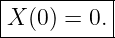
27 Fixed-free string
Now suppose
is fixed but
is free in the idealized transverse sense.
The fixed end requires
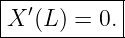
A free end has zero transverse force.
For small slope this gives
With
the free-end condition requires
Thus
Therefore
Only odd multiples of the fundamental occur.
28 Free-free string and the zero mode
For ideal free ends,
There is a constant mode
with
It corresponds to uniform transverse translation in the idealized mathematical model.
The remaining modes have
Boundary conditions determine the spectrum just as constraints determine normal modes in
finite-dimensional mechanics.
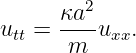
29 Discrete chain to continuous string
M06-06 derived the discrete chain equation
For slow spatial variation,
Thus
The string equation has
Both have the same continuum form:

Figure 8. The oscillator-chain second difference becomes a spatial second derivative in the
long-wavelength limit. Finite-dimensional normal coordinates become the standing-wave normal
modes of a continuous string.
30 Why the continuous spectrum is still discrete on a finite string
The string has infinitely many degrees of freedom because
is defined at continuously many positions.
Yet a finite string with boundary conditions has discrete allowed
The reason is not spatial discreteness.
It is the boundary-value eigenproblem.
Only certain spatial functions satisfy both the differential equation and the endpoint
conditions.
Thus:
- discrete lattices can have discrete or nearly continuous allowed k values depending on
size and boundary conditions,
- continuous media can have discrete normal frequencies when confined to finite domains.
31 Normal modes versus traveling waves
A normal mode of a finite fixed string is naturally represented as a standing wave.
A traveling wave is more natural on an unbounded string or before boundary reflections are
combined.
The two descriptions are related.
A standing mode can be decomposed into equal-frequency left- and right-traveling waves.
Conversely, repeated reflection of traveling waves from boundaries builds the standing-wave
normal-mode structure.
32 Common mistakes
- Using mass density per volume instead of linear mass density μ for the ideal string.
- Forgetting the small-slope approximation in the derivation.
- Treating the tension’s horizontal and transverse components as independently constant.
- Writing c = T∕μ instead of c =
 .
.
- Confusing traveling-wave speed with transverse material-point speed.
- Assuming a standing-wave pattern propagates along the string.
- Forgetting that fixed boundaries require zero displacement.
- Using kn = 2nπ∕L instead of nπ∕L for fixed-fixed modes.
- Confusing angular frequency ωn with ordinary frequency fn.
- Forgetting the factor of 2 in fn = nc∕(2L).
- Calling every Fourier component a distinct physical string rather than a mode of one
string.
- Projecting initial displacement but forgetting initial velocity.
- Assuming all pluck positions excite all harmonics.
- Forgetting that modal mass depends on mode normalization.
- Applying fixed-fixed boundary conditions to fixed-free or free-free problems.
33 Practice exercises
- Derive the transverse force on a short string element and obtain the wave equation.
- Verify dimensionally that c =
 has units of speed.
- Show directly that f(x − ct) satisfies the wave equation.
- Derive the standing-wave form from two counter-propagating sinusoidal waves.
- Use separation of variables to derive the fixed-fixed spatial and temporal equations.
- Derive kn = nπ∕L and fn = nc∕(2L).
- Find the nodes and antinodes of mode n.
- Prove sine-mode orthogonality over 0 ≤ x ≤ L.
- Derive the modal coefficient An from an arbitrary initial displacement.
- Derive the modal coefficient Bn from an arbitrary initial velocity.
- Derive the triangular-pluck coefficients.
- Show that a midpoint pluck excites only odd harmonics.
- Derive the total string energy and show that modal cross terms vanish.
- Derive the fixed-free spectrum.
- Explain how the discrete-chain continuum limit and the finite-string normal modes fit
into one common normal-mode framework.
34 Summary
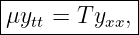
For a uniform stretched string,
or
A fixed-fixed string has normal modes
with
and
An arbitrary fixed-end motion is
| y(x,t) | = ∑
n=1∞![[A cos ω t + B sin ω t]
n n n n](https://images.physicslibrary.org/cache/objects/1502/make4ht/ContinuousStringsStandingWavesAndNormalModes165x.png) | (170)
|
| × sin  , , | (171) |
where
and
The continuum field therefore decomposes into infinitely many independent harmonic normal
coordinates.
This extends the normal-mode machinery from discrete mechanics directly into wave
physics.
References
References
[1] PhysicsLibrary, M06-07, Diatomic Oscillator Chains and Acoustic and Optical
Branches.
[2] PhysicsLibrary, M06-06, Discrete Oscillator Chains and Dispersion.
[3] PhysicsLibrary, M06-05, Small Oscillations and the Normal-Mode Eigenvalue
Problem.
[4] A. P. French, Vibrations and Waves, W. W. Norton, 1971.
[5] J. R. Taylor, Classical Mechanics, University Science Books, 2005.










![∘ ------
--N---
[c] = kg∕m = m∕s.](https://images.physicslibrary.org/cache/objects/1502/make4ht/ContinuousStringsStandingWavesAndNormalModes21x.png)










![y = A [cos(kx − ωt) − cos(kx + ωt)].](https://images.physicslibrary.org/cache/objects/1502/make4ht/ContinuousStringsStandingWavesAndNormalModes34x.png)







































![|--------------------------|
| 1∫ L[ ] |
|E = -- μy2t + T y2x dx.|
------2--0------------------](https://images.physicslibrary.org/cache/objects/1502/make4ht/ContinuousStringsStandingWavesAndNormalModes126x.png)

![|------------------------|
| μL [ ] |
|En = --- Q˙2n + ω2nQ2n .|
--------4----------------](https://images.physicslibrary.org/cache/objects/1502/make4ht/ContinuousStringsStandingWavesAndNormalModes129x.png)