Coupled Oscillators and Normal Modes
A single ideal oscillator has one displacement coordinate and one natural frequency.
A system with several interacting degrees of freedom behaves differently.
Its coordinates are coupled, and the system generally possesses several special collective patterns of
motion called normal modes.
In a normal mode:
- every coordinate oscillates at the same angular frequency,
- the ratios of the coordinate amplitudes remain fixed,
- the entire many-coordinate system behaves like one effective harmonic oscillator.
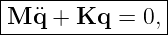
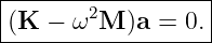
The central linear equation is
where
The normal-mode ansatz
gives
A nonzero mode shape
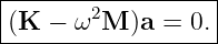
exists only when
This is a generalized eigenvalue problem.
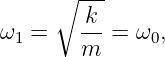
The eigenvalues are
and the eigenvectors are the corresponding mode shapes.
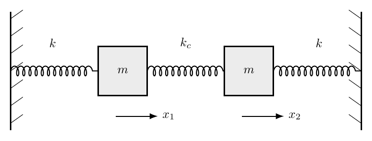
Figure 1. Two equal masses attached to outer springs and coupled by a middle spring form the
standard two-degree-of-freedom oscillator. The coupling spring makes the motion of one mass
influence the other.
1 Two identical masses with three springs
Consider two equal masses
with displacements
Each mass is attached to a wall by a spring of constant
and the masses are joined by a coupling spring of constant
When mass 1 moves by
and mass 2 by
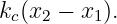
the extension of the coupling spring is
The coupling force on mass 1 is
The coupling force on mass 2 is
2 Equations of motion
For mass 1,
Thus
For mass 2,
Thus
Each equation contains both coordinates.
That is the defining feature of a coupled system.
3 Matrix form
Define
Then
and
The equations become
4 Normal-mode ansatz
Seek a motion in which both coordinates oscillate at one common frequency:
where
is a constant vector.
Then
Substitution gives
For this system,
5 Characteristic equation
A nonzero vector
requires
Thus
Factor:
| 0 | = ![[ 2 ]
k + kc − m ω − kc](https://images.physicslibrary.org/cache/objects/1494/make4ht/CoupledOscillatorsAndNormalModes31x.png) | (32)
|
| ×![[ ]
k + kc − m ω2 + kc](https://images.physicslibrary.org/cache/objects/1494/make4ht/CoupledOscillatorsAndNormalModes32x.png) . . | (33) |
Therefore
and
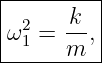
The coupled two-mass system has two natural frequencies.
6 First normal mode: in-phase motion
For
the eigenvalue equation becomes
Therefore
A convenient normalized mode shape is
Both masses move together.
The coupling spring is not stretched because
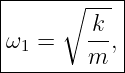
Therefore the coupling stiffness does not contribute to this mode’s restoring force.
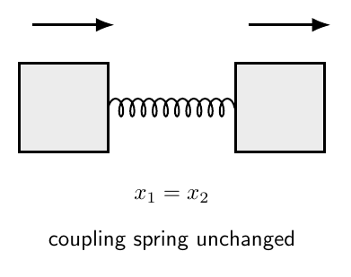
Figure 2. In the symmetric or in-phase normal mode, both masses move together. The coupling
spring retains its equilibrium length, giving ω1 =  .
.
7 Second normal mode: out-of-phase motion
For
the eigenvalue equation gives
Thus
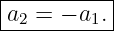
A normalized mode shape is
The masses move oppositely.
The coupling spring changes length strongly, increasing the restoring stiffness.
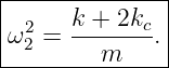
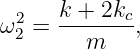
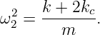
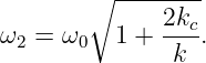
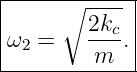
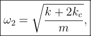
Therefore
for
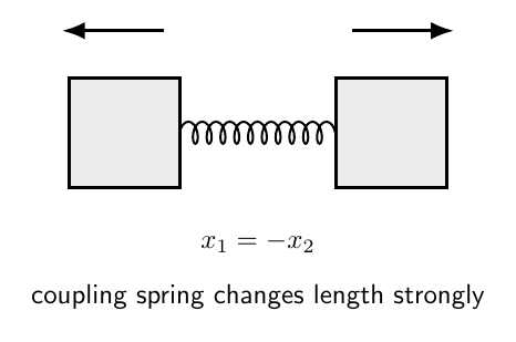
Figure 3. In the antisymmetric or out-of-phase normal mode, the masses move oppositely. The
coupling spring stretches and compresses strongly, increasing the mode frequency to
ω2 =  .
.
8 Normal coordinates
The original coordinates
are physically intuitive but dynamically coupled.
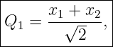
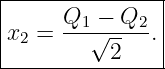
Define instead
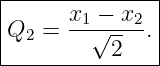
and
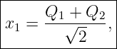
These are the normal coordinates.
The inverse transformation is
and
The coordinate
measures the in-phase motion.
The coordinate
measures the out-of-phase motion.
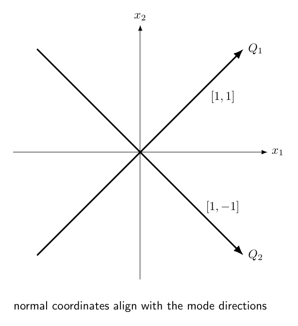
Figure 4. The transformation from physical coordinates (x1,x2) to normal coordinates (Q1,Q2)
rotates the coordinate description into the two mode directions.
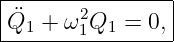
9 Decoupling the equations
Add the two physical-coordinate equations:
Therefore
where
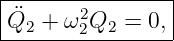
Subtract the second physical equation from the first:
Therefore
where
The coupled system has become two independent harmonic oscillators.
This is the central purpose of normal coordinates.
10 General solution in normal coordinates
Each normal coordinate has its own SHO solution:
and
Transforming back,
and
A general motion is therefore a superposition of normal modes.
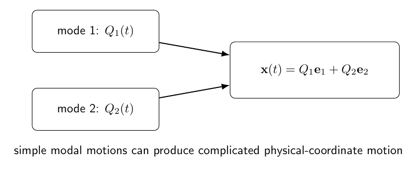
Figure 5. A general coupled motion is a superposition of the system’s normal modes. Each normal
coordinate evolves independently at its own Normal frequency.
11 Initial conditions determine modal amplitudes
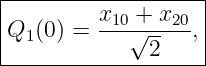
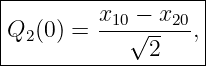
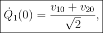
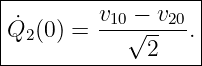
Suppose
and
Then
and similarly
Each modal initial state then determines its own amplitude and phase using the SHO results from
M06-01.
12 Example 1: one mass displaced and released
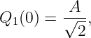
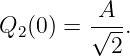
Suppose
and
Then
and
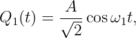
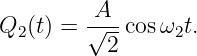
Because both modal velocities initially vanish,
and
Therefore
and
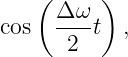
13 Beats and energy exchange
Use
Then
Similarly,
up to an overall sign convention.
When the coupling is weak,
is small.
The fast oscillation is modulated by a slow envelope.
Motion appears to transfer back and forth between the two masses.
This is the coupled-oscillator origin of beats and energy exchange.
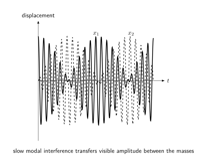
Figure 6. When the two normal frequencies are close, a displacement initially concentrated on one
mass evolves into a slow exchange of oscillation amplitude between the two masses.
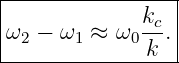
14 Weak-coupling frequency splitting
If
then
and
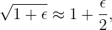
Using
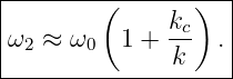
Thus
The normal-frequency splitting is therefore a direct measure of weak coupling strength.
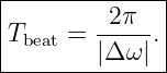
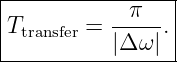
15 Beat time scale
The slow envelope contains
where
The envelope magnitude repeats after
Complete transfer from one mass to the other occurs on the half-beat time scale
16 Energy of the two-mass system
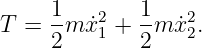
The kinetic energy is
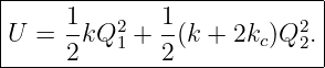
The potential energy is
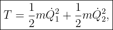
Using the normal-coordinate transformation,
one obtains
and
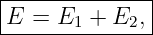
Therefore
where
and
The normal coordinates diagonalize the energy as well as the equations of motion.
17 Why normal modes do not exchange energy
In the ideal linear conservative system,
and
satisfy independent SHO equations.
Thus
and
are separately conserved.
The apparent energy exchange between the physical masses is not energy transfer between normal
modes.
It is interference between fixed-energy modal contributions when transformed back into the
physical coordinates.
This distinction is important.
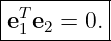
18 Orthogonality of the equal-mass mode shapes
The two mode shapes are
and
Their ordinary dot product is
For equal masses,
so ordinary orthogonality and mass orthogonality are equivalent.
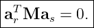
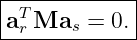
19 General mass orthogonality
For a general conservative system,
and
Assume
and
Multiply the first equation on the left by
and the second on the left by
Symmetry gives
Since
For distinct frequencies,
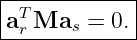
Distinct normal modes are orthogonal with respect to the mass matrix.
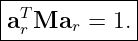
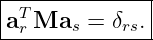
20 Mass normalization
A mode shape can be multiplied by any nonzero constant without changing the physical
mode.
A convenient convention is
Then the mode shapes are mass normalized.
For mass-normalized modes,
This normalization is especially useful for many-degree-of-freedom systems.
21 General modal transformation
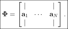
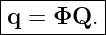
Collect the normal-mode vectors into the modal matrix
Write
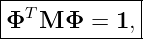
For mass-normalized modes,
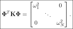
and
Therefore
The coupled physical-coordinate equations become independent modal equations.
22 Generalized eigenvalue problem
For
degrees of freedom,
Use
Then
The normal frequencies satisfy
This is the standard small-oscillation eigenvalue problem.
23 Mass-weighted coordinates
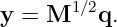
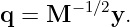
When
is positive definite, define
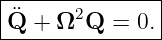
Then
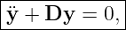
The equations become
where
If
is symmetric, then
is symmetric.
The generalized eigenvalue problem has therefore been converted into an ordinary symmetric
eigenvalue problem.
24 Zero modes
Not every normal frequency must be positive.
Consider two equal masses connected only to each other by a spring, with no springs to fixed
walls.
The equations are
| mẍ1 + kc(x1 − x2) | = 0, | (137)
|
| mẍ2 + kc(x2 − x1) | = 0. | (138) |
The in-phase mode
does not stretch the spring.
Thus there is no restoring force.
Its frequency is
This is a zero mode.
It represents uniform translation of the entire system.
The out-of-phase mode has
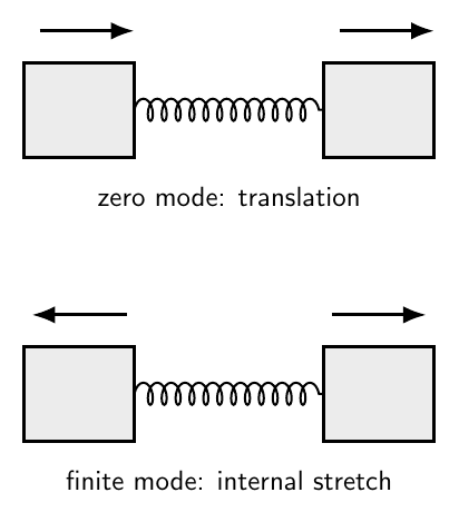
Figure 7. Two masses connected only to each other possess a zero-frequency in-phase mode
corresponding to rigid translation and a finite-frequency internal stretching mode.
25 Zero modes and continuous symmetry
The zero mode exists because translating both masses by the same amount does not change the
spring extension or potential energy.
This reflects translational symmetry.
More generally, zero modes often arise when a continuous change of configuration costs no
potential energy.
Examples include:
- uniform translation of an isolated system,
- rigid rotation of a rotationally invariant configuration,
- symmetry motions in more complicated mechanical systems.
26 Unequal masses
Suppose
Then
The normal-mode equation remains
The ordinary Euclidean eigenvectors need not be orthogonal.
Instead, distinct modes satisfy
Thus the mass matrix defines the physically natural inner product.
27 Example 2: numerical equal-mass system
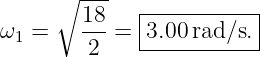
Let
Then
The second frequency is
| ω2 | = 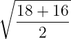 | (148)
|
| =  | (149)
|
| ≈ 4.12 rad∕s. | (150) |
Thus
The corresponding beat time is
| Tbeat | =  | (152)
|
| ≈ 5.59 s. | (153) |
28 Small oscillations of a general mechanical system
Let generalized coordinates be
and let
represent stable equilibrium.
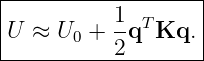
Near equilibrium, the potential energy is approximately quadratic:
The matrix
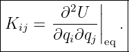
is the Hessian of the potential evaluated at equilibrium:
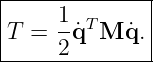
For many systems the kinetic energy near equilibrium is
The linearized equations are then
Thus normal modes are the universal linear description of small oscillations about stable
equilibrium.
29 From finite oscillators to waves
Consider a chain of many identical masses coupled by identical springs.
With
masses, there are
normal modes.
As
becomes large:
- the allowed mode frequencies become dense,
- the mode shapes resemble sampled sine or exponential patterns,
- the system approaches a continuous elastic medium.
The normal modes of a continuous string are Standing Waves.
Thus the mathematics of coupled oscillators is the direct bridge from particle mechanics to wave
physics.
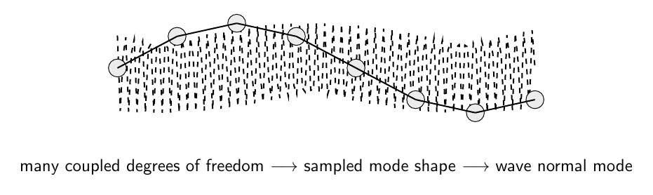
Figure 8. Increasing the number of coupled oscillators produces a family of collective modes. In
the continuum limit, these discrete mode shapes become the normal modes of wave systems.
30 Driven coupled systems
If an external force vector is applied,
In modal coordinates,
for mass-normalized modes.
Thus each normal coordinate behaves like a driven oscillator.
A drive couples strongly to a mode when:
- its frequency is near that mode’s natural frequency,
- its spatial force pattern has a nonzero projection onto that mode shape.
This introduces the idea of modal participation.
31 Damping in coupled systems
With damping,
The undamped normal modes still completely decouple the system only for special damping
structures, such as proportional damping.
General damping can couple modal coordinates again.
Thus the clean normal-mode theory developed here is fundamentally the conservative linear
starting point.
32 Normal modes versus arbitrary motion
A normal mode is not just any oscillatory motion.
A normal mode has:
- one definite angular frequency,
- a fixed coordinate-amplitude ratio,
- a fixed relative phase pattern.
An arbitrary motion generally contains several normal modes simultaneously.
Its physical-coordinate motion can therefore look complicated even though every normal
coordinate follows a simple harmonic equation.
33 Common mistakes
- Assuming coupled coordinates can be solved independently before finding normal
coordinates.
- Confusing physical coordinates with normal coordinates.
- Treating the determinant condition alone as sufficient without finding the
corresponding eigenvectors.
- Forgetting that a mode shape is defined only up to an overall scale.
- Assuming the higher-frequency mode must always be in phase.
- Forgetting that the coupling spring is unstretched in the symmetric equal-mass mode.
- Forgetting that the coupling spring contributes twice to the effective stiffness of the
antisymmetric equal-mass mode.
- Confusing energy exchange between physical masses with energy exchange between
ideal normal modes.
- Using ordinary dot-product orthogonality for unequal masses instead of mass
orthogonality.
- Assuming every mode frequency must be nonzero.
- Missing zero modes associated with continuous symmetries.
- Forgetting that a general motion is a superposition of all excited normal modes.
- Using the normal-mode eigenvectors without transforming initial velocities as well as
initial displacements.
- Assuming damping always preserves exact modal decoupling.
- Missing the connection between a long oscillator chain and wave normal modes.
34 Practice exercises
- Derive the coupled equations for the equal-mass three-spring system.
- Construct the mass and stiffness matrices.
- Derive the characteristic equation and both normal frequencies.
- Find and normalize the two mode shapes.
- Explain physically why the symmetric mode frequency is independent of kc.
- Explain physically why the antisymmetric mode has the larger frequency.
- Derive the normal-coordinate transformation and its inverse.
- Show directly that the equations decouple in Q1 and Q2.
- Show that kinetic and potential energy also diagonalize in the normal coordinates.
- For one mass initially displaced and the other at rest, derive x1(t) and x2(t).
- Derive the beat time and complete-transfer time from ω2 − ω1.
- Derive the weak-coupling frequency splitting.
- Prove the mass-orthogonality relation for two distinct modes.
- Derive the zero and nonzero frequencies of two free masses connected only by one
spring.
- Show how mass-weighted coordinates convert the generalized eigenvalue problem into
an ordinary symmetric eigenvalue problem.
35 Summary
Coupled linear oscillators satisfy
A normal mode has the form
Therefore
The allowed frequencies satisfy
For two equal masses attached to outer springs
and coupled by
with mode shape
and
with mode shape
Normal coordinates decouple both the equations of motion and the quadratic energy.
For distinct modes of a general conservative system,
The same eigenvalue structure extends from a few coupled masses to the normal modes of
continuous wave systems.
References
References
[1] PhysicsLibrary, M06-03, Driven Harmonic Motion and Resonance.
[2] PhysicsLibrary, M06-02, Damped Harmonic Motion.
[3] PhysicsLibrary, M06-01, Simple Harmonic Motion.
[4] A. P. French, Vibrations and Waves, W. W. Norton, 1971.
[5] J. R. Taylor, Classical Mechanics, University Science Books, 2005.














![[ ]
x1
x = x2 .](https://images.physicslibrary.org/cache/objects/1494/make4ht/CoupledOscillatorsAndNormalModes19x.png)
![|--------[----]--|
|M = m 1 0 ,|
| 0 1 |
-----------------](https://images.physicslibrary.org/cache/objects/1494/make4ht/CoupledOscillatorsAndNormalModes20x.png)
![|-----[--------------]-|
| k + kc − kc |
K = − k k + k .|
-----------c--------c---](https://images.physicslibrary.org/cache/objects/1494/make4ht/CoupledOscillatorsAndNormalModes21x.png)


![[ ]
a = a1
a2](https://images.physicslibrary.org/cache/objects/1494/make4ht/CoupledOscillatorsAndNormalModes24x.png)


![[ ][ ]
k + kc − mω2 − kc a1
− kc k + kc − mω2 a2 = 0.](https://images.physicslibrary.org/cache/objects/1494/make4ht/CoupledOscillatorsAndNormalModes27x.png)






![---------------
| [ ] |
|e1 = √1-- 1 .|
--------2--1---|](https://images.physicslibrary.org/cache/objects/1494/make4ht/CoupledOscillatorsAndNormalModes38x.png)


![|---------[---]--|
| -1-- 1 |
|e2 = √2-- − 1 .|
-----------------](https://images.physicslibrary.org/cache/objects/1494/make4ht/CoupledOscillatorsAndNormalModes44x.png)






























![[ ]
-1-- 1
e1 = √ -- 1 ,
2](https://images.physicslibrary.org/cache/objects/1494/make4ht/CoupledOscillatorsAndNormalModes105x.png)
![[ ]
-1-- 1
e2 = √ 2 − 1 .](https://images.physicslibrary.org/cache/objects/1494/make4ht/CoupledOscillatorsAndNormalModes106x.png)


















![[ ]
m1 0
M = 0 m2 .](https://images.physicslibrary.org/cache/objects/1494/make4ht/CoupledOscillatorsAndNormalModes142x.png)

















![[--]-|
| 1 |
| 1 ,|
------](https://images.physicslibrary.org/cache/objects/1494/make4ht/CoupledOscillatorsAndNormalModes171x.png)
![[----]-|
| 1 .|
| − 1 |
--------](https://images.physicslibrary.org/cache/objects/1494/make4ht/CoupledOscillatorsAndNormalModes173x.png)