Discrete Oscillator Chains and Dispersion

(Topic)

Discrete Oscillator Chains and Dispersion

M06-04 and M06-05 showed that a finite linear mechanical system can be decomposed into normal modes.

A chain of many coupled oscillators applies the same idea repeatedly in space.

The simplest model is a one-dimensional monatomic lattice:

identical masses m,
equilibrium spacing a,
identical nearest-neighbor springs of constant κ,
one longitudinal displacement u_n(t) for the mass at lattice site n.

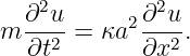
The equation of motion is

|------------------------------| |m ¨un = κ (un+1 − 2un + un− 1).| -------------------------------

(1)

This is the discrete analogue of a wave equation.

Its normal modes are traveling lattice waves.

Unlike the ideal continuous wave equation, however, the lattice does not generally have a linear relation between frequency and wave number.

Instead it has a dispersion relation.

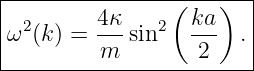
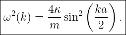
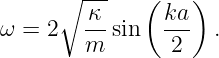
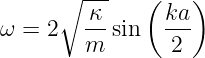
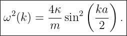
For the monatomic nearest-neighbor chain,

|---------------(---)---| | 2 4κ- 2 ka- | ω (k ) = m sin 2 . | -------------------------

(2)

This one equation contains the long-wavelength continuum limit, a maximum lattice frequency, wave-number periodicity, phase velocity, group velocity, and the onset of lattice dispersion.

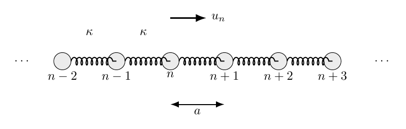
Figure 1. A monatomic oscillator chain consists of identical masses separated by equilibrium spacing a and connected by identical nearest-neighbor springs of constant κ. The displacement of lattice site n is u_n(t).

1 Force on one lattice mass

Consider the mass at site

n.

(3)

The spring to the right changes length by

un+1 − un.

(4)

It therefore exerts the force

Fn,right = κ(un+1 − un).

(5)

The spring to the left changes length by

un − un−1.

(6)

Its force on mass

n

(7)

Fn,left = − κ(un − un −1).

(8)

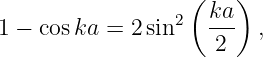
The total force is

F_n	= κ(u_n+1 − u_n) − κ(u_n − u_n−1)	(9)
	= κ(u_n+1 − 2u_n + u_n−1).	(10)

Newton’s second law gives

|-----------------------------| m ¨un = κ(un+1 − 2un + un− 1). | -------------------------------

(11)

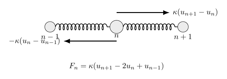
Figure 2. The net restoring force on mass n is the difference between the right-spring and left-spring extensions. The resulting second spatial difference is the discrete counterpart of curvature in a continuous medium.

2 Discrete second difference

The combination

un+1 − 2un + un− 1

(12)

is the centered second difference.

It measures how strongly the displacement at site

n

(13)

differs from the local average of its neighbors.

un+1 = un = un −1,

(14)

the springs are not differentially stretched and the net restoring force vanishes.

This is the discrete analogue of a continuous field with zero curvature.

3 Normal-mode trial solution

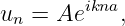
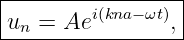
Because the chain is translationally repetitive, try a mode of the form

|-------------------| un (t) = Aei(kna−ωt). | ---------------------

(15)

The physical displacement is the real part.

The neighboring displacements are

u = u eika, n+1 n

(16)

and

u = u e−ika. n− 1 n

(17)

Also,

2 u¨n = − ω un.

(18)

Substitute into the lattice equation:

2 ( ika − ika) − m ω un = κ e − 2 + e un.

(19)

Using

eika + e−ika = 2coska,

(20)

− m ω2 = 2κ(cos ka − 1).

(21)

Since

( ) 2 ka- 1 − coska = 2sin 2 ,

(22)

|-----------------------| | 4κ ( ka) | ω2 (k ) = ---sin2 --- . | ---------m--------2------

(23)

4 Dispersion relation

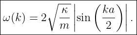
Choose the nonnegative frequency:

|--------∘----|----------|-| | κ | ( ka ) | | |ω(k) = 2 --||sin --- ||.| ------------m--------2-----

(24)

A relation of the form

ω = ω(k)

(25)

is called a dispersion relation.

ω

(26)

is proportional to

|k|,

(27)

all wavelengths propagate with the same characteristic speed and the medium is nondispersive.

The lattice relation is nonlinear in

k.

(28)

Therefore the discrete chain is dispersive except in its long-wavelength limit.

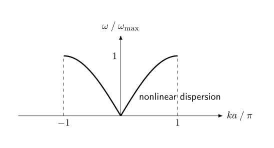
Figure 3. The monatomic-chain dispersion relation is approximately linear near k = 0 but bends over and reaches its maximum frequency at the edge of the first Brillouin zone, |k| = π∕a.

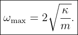
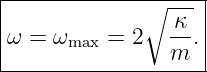
5 Maximum frequency

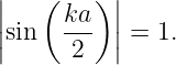
The sine magnitude cannot exceed unity.

Therefore

|--------------| | ∘ κ--| |ωmax = 2 --.| ------------m---

(29)

The maximum occurs when

| | | ( ka) | ||sin --- || = 1. 2

(30)

Within the first Brillouin zone this is

|--------| ||k | = π-. ------a---

(31)

Thus a discrete lattice has an upper frequency for this branch.

The continuous ideal wave equation has no corresponding lattice cutoff.

6 Wave-number equivalence

At the lattice sites,

ei(k+2π∕a)na = eiknaei2πn.

(32)

Since

ei2πn = 1

(33)

for integer

n,

(34)

|----------------| | 2π | k and k + ---| ---------------a--

(35)

describe the same pattern on the discrete lattice.

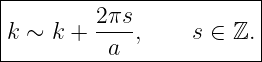
More generally,

|------------------------| |k ∼ k + 2πs-, s ∈ ℤ. | ----------a---------------

(36)

This is reciprocal-lattice periodicity.

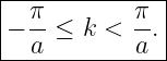
7 First Brillouin zone

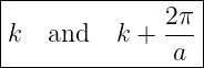
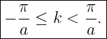
Because wave numbers separated by

2π ∕a

(37)

are equivalent on the monatomic lattice, one complete set of distinct wave numbers can be chosen as

|--π--------π--| |− --≤ k < --.| ---a--------a--|

(38)

This interval is the first Brillouin zone in one dimension.

Its width is

|----| |2π- | | a .| -----

(39)

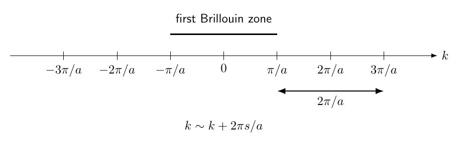
Figure 4. Wave numbers separated by a reciprocal-lattice vector 2π∕a give identical phase factors at every lattice site. Distinct lattice modes can therefore be represented within the first Brillouin zone.

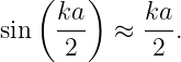
8 Long-wavelength limit

Suppose

|ka| ≪ 1.

(40)

Then

( ) ka- ka- sin 2 ≈ 2 .

(41)

Therefore

ω	≈ 2	(42)
	= a\|k\|.	(43)

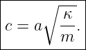
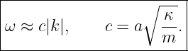
Define

|-----∘----| | κ | c = a --.| --------m---

(44)

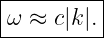
Then

|--------| ω ≈ c|k |.| ----------

(45)

The lattice becomes approximately nondispersive at wavelengths much larger than

a.

(46)

9 Continuum limit from Taylor expansion

Let

u (t) ≈ u(x, t), x = na, n

(47)

for a field that varies slowly over one lattice spacing.

Expand:

u(x + a,t)	= u + a + + ,	(48)
u(x − a,t)	= u − a + + .	(49)

Adding,

2 u(x + a) − 2u(x ) + u(x − a ) ≈ a2∂-u-. ∂x2

(50)

The lattice equation becomes

∂2u- 2∂2u- m ∂t2 = κa ∂x2.

(51)

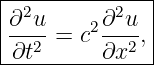
Thus

|-2--------2---| |∂-u-= c2∂-u-,| -∂t2------∂x2--|

(52)

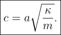
with

|----------| | ∘ κ | c = a --.| --------m---

(53)

The continuous wave equation emerges as the long-wavelength limit of the discrete chain.

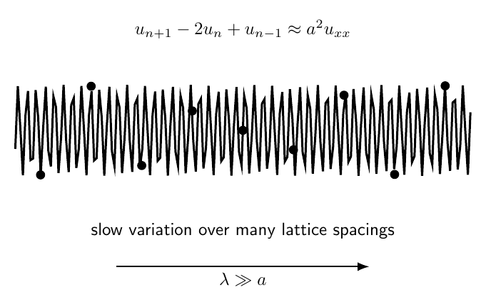
Figure 8. When the displacement varies slowly over many lattice spacings, the centered second difference approaches a²∂²u∕∂x², and the discrete oscillator chain approaches the continuous wave equation.

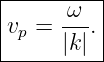
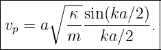
10 Phase velocity

For a sinusoidal mode,

|-----ω--| vp = --.| ------|k|--

(54)

For

0 < k ≤ π∕a,

(55)

--- ∘ κ ( ka) ω = 2 -- sin --- . m 2

(56)

Hence

|------∘---------------| | κ sin(ka∕2) | |vp = a ------------.| ----------m---ka-∕2----

(57)

Thus

vp → c

(58)

k → 0.

(59)

For finite

ka,

(60)

the phase velocity depends on wave number.

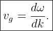
11 Group velocity

A localized wave packet requires a range of nearby wave numbers.

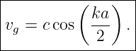
Its envelope propagates approximately at the group velocity

|---------| | d-ω | vg = dk. | -----------

(61)

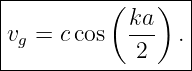
For

0 < k < π∕a,

(62)

v_g	=	(63)
	= a cos .	(64)

Therefore

|------------------| | ( ) | |vg = ccos ka- . | -------------2-----

(65)

At long wavelength,

v → c. g

(66)

At the zone boundary,

|--------| -vg-→--0.|

(67)

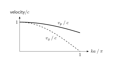
Figure 5. Both phase and group velocities approach the continuum speed c as k → 0. The group velocity falls to zero at the zone boundary because the dispersion curve becomes horizontal there.

12 Why group velocity matters

A single infinite sinusoidal mode fills all space and has no localized envelope.

Physical disturbances are usually superpositions of modes.

For a narrow packet centered near

k0,

(68)

the envelope travels approximately at

vg(k0).

(69)

In many conservative wave systems, group velocity is also closely connected to the transport of energy.

Thus the shape of

ω (k)

(70)

determines how disturbances propagate through the lattice.

13 Wave-packet dispersion

ω (k)

(71)

were exactly linear, nearby Fourier components would have the same group velocity and a narrow packet would preserve its shape.

For the lattice,

d2ω --2-⁄= 0 dk

(72)

away from the continuum limit.

Different components then travel with slightly different group velocities.

The packet can spread or distort.

This is the physical meaning of dispersion.

14 Zone-boundary mode

π k = -, a

(73)

the lattice phase factor is

eikna = eiπn = (− 1)n.

(74)

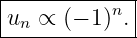
Therefore neighboring masses move in opposite directions:

|------------| |un ∝ (− 1)n.| --------------

(75)

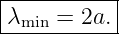
This mode has

|------------------| | ∘ κ--| ω = ωmax = 2 --.| ----------------m---

(76)

Its shortest distinct lattice wavelength is

|----------| -λmin =-2a.-

(77)

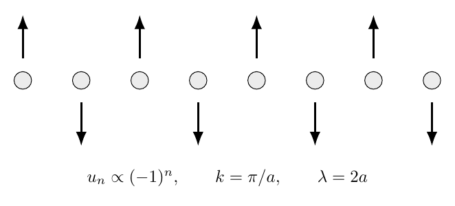
Figure 7. At the Brillouin-zone boundary, neighboring masses move exactly out of phase. The corresponding lattice wavelength is 2a, the shortest distinct wavelength that can be represented on the monatomic lattice.

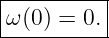
15 The zero-frequency mode

k = 0,

(78)

all sites have the same displacement:

un = Ae −iωt.

(79)

The dispersion relation gives

|----------| |ω (0 ) = 0.| -----------

(80)

For a free or periodic chain, this is uniform translation.

No spring is stretched, so there is no restoring force.

This is the extended-chain version of the zero mode introduced in M06-04 and M06-05.

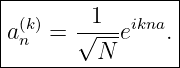
16 Periodic chain of N masses

Consider

N

(81)

masses with periodic boundary condition

u = u . n+N n

(82)

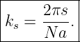
For the traveling mode

ikna un = Ae ,

(83)

periodicity requires

ikNa e = 1.

(84)

Therefore

kN a = 2πs,

(85)

where

s

(86)

is an integer.

Thus

|----------| | 2πs- | |ks = N a .| -----------

(87)

Only

N

(88)

distinct wave numbers occur within one Brillouin zone.

These are the

N

(89)

normal modes of the

N

(90)

degree-of-freedom periodic chain.

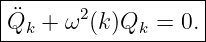
17 Fourier coordinates are normal coordinates

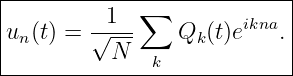
For a periodic chain, write the discrete Fourier expansion

|---------1--∑--------------| un (t) = √---- Qk(t)eikna. | | N k | ----------------------------|

(91)

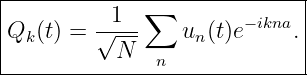
The inverse transform is

|----------1--∑--------------| |Qk(t) = √---- un (t)e− ikna.| | N n | ------------------------------

(92)

The Fourier amplitudes

Qk

(93)

are the normal coordinates of the translationally invariant chain.

Substitution into the equations gives, mode by mode,

|------------------| Q¨k + ω2(k)Qk = 0.| --------------------

(94)

Thus the discrete Fourier transform diagonalizes the chain dynamics.

18 Connection to the matrix eigenvalue problem

For a finite periodic chain,

M = m1.

(95)

The stiffness matrix is circulant.

Its eigenvectors are the discrete Fourier vectors

|----------------| | 1 | |a(kn) = √----eikna.| ---------N--------

(96)

The generalized eigenvalue equation

2 Ka = ω Ma

(97)

therefore becomes exactly the lattice dispersion relation.

This is the many-site version of the normal-mode construction developed in M06-05.

19 Standing waves from opposite wave numbers

Because

ω (k) = ω(− k),

(98)

the modes at

+k

(99)

and

− k

(100)

have the same frequency.

Their linear combinations can form real Standing Waves:

|--------------------| un ∝ cos(kna) cosωt,| ----------------------

(101)

|--------------------| un ∝ sin (kna )cos ωt.| ----------------------

(102)

The traveling-wave and standing-wave descriptions are therefore alternative bases within the same degenerate

±k

(103)

subspace.

20 Finite chain with fixed ends

Now consider

N

(104)

moving masses between fixed endpoints:

u0 = 0, uN+1 = 0.

(105)

Use the standing-wave form

un = A sin (kna )cos ωt.

(106)

The first boundary condition is automatic.

The second requires

sin[k(N + 1 )a ] = 0.

(107)

Therefore

|--------------------------------| | ---rπ---- | kr = (N + 1)a , r = 1,...,N. | ----------------------------------

(108)

The corresponding frequencies are

|------∘--------[---------]--| | κ- ---rπ---- | |ωr = 2 m sin 2(N + 1) .| -----------------------------

(109)

There are exactly

N

(110)

normal modes.

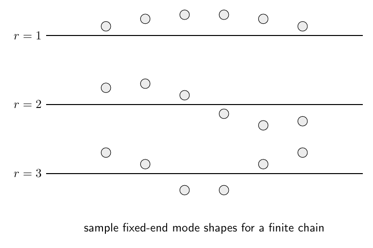
Figure 6. A finite fixed-end chain has discrete standing-wave mode shapes. Higher mode number means shorter wavelength and higher frequency, until the lattice-scale zone-boundary pattern is approached.

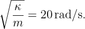
21 Example 1: four masses with fixed ends

Let

N = 4, m = 0.250 kg, κ = 100 N ∕m.

(111)

Then

∘ --- κ- m = 20 rad∕s.

(112)

The four frequencies are

( rπ) ωr = 40 sin 10 rad∕s.

(113)

Thus

ω₁	≈ 12.36 rad∕s ,	(114)
ω₂	≈ 23.51 rad∕s ,	(115)
ω₃	≈ 32.36 rad∕s ,	(116)
ω₄	≈ 38.04 rad∕s.	(117)

All lie below the infinite-chain maximum

ωmax = 40 rad∕s.

(118)

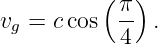
22 Example 2: group velocity

Let

a = 0.10 m, κ = 400N ∕m, m = 1.00 kg.

(119)

The continuum speed is

∘ -κ- |----------| c = a -- = 0.10(20 ) =|2.00m ∕s. | m -----------

(120)

π ka = --, 2

(121)

(π ) vg = ccos -- . 4

(122)

Therefore

|-----√------------------| -vg =--2-m-∕s ≈-1.41m-∕s.-

(123)

The group velocity is already below the long-wavelength speed.

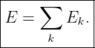
23 Energy of the chain

For a periodic chain, the mechanical energy is

|------------------------------------| | ∑ [ 1 1 ] | |E = -m ˙u2n + --κ(un+1 − un)2 .| | n 2 2 | -------------------------------------

(124)

In Fourier normal coordinates, the quadratic energy separates into independent modal contributions.

Schematically,

|-----∑------| |E = Ek. | | k | --------------

(125)

Each normal mode is an independent harmonic oscillator.

A localized wave packet contains many

k

(126)

modes, and their differing phases and group velocities determine how energy moves through the chain.

24 Discrete sampling and the shortest wavelength

The lattice samples displacement only at positions

xn = na.

(127)

Two continuous sinusoids whose wave numbers differ by

2π ∕a

(128)

give the same values at every sample point.

This is mathematically analogous to aliasing in sampled-data systems.

The first Brillouin zone is therefore the natural nonredundant wave-number interval.

The zone-boundary wavelength

λ = 2a

(129)

is the shortest distinct sinusoidal pattern on the lattice.

25 Continuum approximation error

The exact relation is

∘ --- ( ) κ- ka- ω = 2 m sin 2

(130)

for

0 ≤ k ≤ π∕a.

(131)

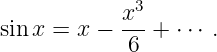
Expand the sine:

x3- sinx = x − 6 + ⋅⋅⋅ .

(132)

Then

= ck

(133)

Thus the leading correction to the nondispersive continuum relation is of order

|------| |(ka)2.| -------

(134)

The continuum model improves rapidly when the wavelength is large compared with

a.

(135)

26 Mode counting

A chain with

N

(136)

independent scalar displacements has

N

(137)

normal modes.

The wave description does not create additional degrees of freedom.

Instead, it relabels the same finite-dimensional modal basis by wave number.

For a very large periodic chain, the allowed

k

(138)

values become closely spaced and the normal-mode spectrum appears nearly continuous.

27 What dispersion means physically

The word dispersion refers to wave-number-dependent propagation.

In this chain:

different wave numbers have different phase velocities,
different wave numbers have different group velocities,
a localized packet can spread,
the group velocity approaches zero near the zone boundary.

The origin of the dispersion is the discrete microstructure.

At wavelengths much longer than the lattice spacing, that microstructure is not resolved and the medium appears continuous.

28 Preview of a two-mass basis

The monatomic chain has one displacement degree of freedom per primitive cell and therefore one frequency branch.

If each cell contains two inequivalent masses, the eigenvalue problem becomes two-dimensional for every

k.

(139)

Two branches result:

an acoustic branch,
an optical branch.

That extension is developed in M06-07.

29 Common mistakes

Treating the lattice equation as if neighboring displacements were independent forcing terms.
Losing the factor of 2 when converting 1 − cos ka to sin ²(ka∕2).
Confusing lattice spacing a with oscillation amplitude.
Assuming ω is proportional to k for all wavelengths.
Forgetting that k and k + 2π∕a are equivalent on the lattice.
Counting wave numbers outside the first Brillouin zone as new independent modes.
Confusing phase velocity with group velocity.
Assuming group velocity remains equal to c near the zone boundary.
Forgetting that v_g = 0 at |k| = π∕a.
Calling λ < 2a a distinct lattice wavelength.
Forgetting that k = 0 is a zero-frequency translation mode for a free or periodic monatomic chain.
Applying the periodic-chain wave-number quantization to a fixed-end chain.
Forgetting the N + 1 in the fixed-end result k_r = rπ∕[(N + 1)a].
Confusing the number of lattice sites with the number of reciprocal-lattice periods.
Assuming a dispersive wave packet preserves its shape exactly.

30 Practice exercises

Derive the force on lattice site n from its two neighboring springs.
Starting from the complex traveling-wave ansatz, derive the monatomic dispersion relation.
Show explicitly that k and k + 2π∕a produce identical lattice displacements.
Identify the first Brillouin zone and explain why it contains a complete set of distinct wave numbers.
Derive the maximum lattice frequency and the corresponding mode pattern.
Derive the long-wavelength speed c = a.
Derive the continuum wave equation from Taylor expansions of u(x ± a,t).
Derive the phase velocity as a function of k.
Derive the group velocity and show that it vanishes at the zone boundary.
Show that the leading continuum-dispersion correction is proportional to (ka)².
Derive the allowed wave numbers for a periodic chain of N masses.
Show that the discrete Fourier coordinates decouple the periodic chain equations.
Derive the fixed-end normal modes and frequencies for N masses.
Reproduce all four frequencies in Example 1.
Explain why the monatomic chain has one branch and predict qualitatively what changes when there are two masses per primitive cell.

31 Summary

The monatomic nearest-neighbor chain obeys

|-----------------------------| m ¨un = κ(un+1 − 2un + un− 1). | -------------------------------

(140)

Its traveling normal modes have

|----------------| un = Aei(kna− ωt),| ------------------

(141)

with dispersion relation

|---------------(---)---| | 2 4κ 2 ka | ω (k ) = m--sin 2-- . | -------------------------

(142)

One nonredundant wave-number interval is

|--------------| |− π-≤ k < π-.| ---a--------a--|

(143)

The long-wavelength limit is

|------------------------| | ∘ ---| |ω ≈ c|k|, c = a κ-.| ----------------------m---

(144)

For

0 < k < π∕a,

(145)

|----------(---)---| | ka- | |vg = ccos 2 . | -------------------

(146)

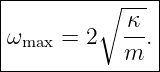
The maximum frequency occurs at the zone boundary:

|--------∘-----| |ω = 2 κ-.| | max m | ----------------

(147)

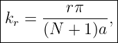
For a fixed-end chain of

N

(148)

masses,

|----------------| |k = ----rπ---, | | r (N + 1)a | -----------------

(149)

and

|------∘---------------------| | κ [ rπ ] | |ωr = 2 --sin --------- .| ----------m------2(N--+-1)---

(150)

The oscillator chain therefore connects the finite-dimensional normal-mode eigenproblem directly to wave propagation and dispersion.

References

[1] PhysicsLibrary, M06-05, Small Oscillations and the Normal-Mode Eigenvalue Problem.

[2] PhysicsLibrary, M06-04, Coupled Oscillators and Normal Modes.

[3] PhysicsLibrary, M06-03, Driven Harmonic Motion and Resonance.

[4] A. P. French, Vibrations and Waves, W. W. Norton, 1971.

[5] C. Kittel, Introduction to Solid State Physics, 8th ed., Wiley, 2005.

[6] J. R. Taylor, Classical Mechanics, University Science Books, 2005.

"Discrete Oscillator Chains and Dispersion" is owned by bloftin.
(view preamble)

Discrete Oscillator Chains and Dispersion