EDL01: Practical Electricity and Measurement for Electrodynamics
Laboratory purpose. Before using instruments to investigate electric fields, magnetic
fields, induction, and electromagnetic waves, we must understand how a measurement
changes the circuit being measured. A voltmeter draws current, an ammeter introduces a
small voltage drop, a signal generator has an output impedance, and an oscilloscope
probe can add capacitance. These effects are small in some experiments and decisive in
others.
This entry develops a reusable measurement method through a sequence of low-voltage
experiments. It is an experimental companion to the EDL00 roadmap and the PhysicsLibrary
Electromagnetism series. It is not a substitute for circuit theory or for the field formulation of
electrodynamics.
At the end of the article, the reader should be able to measure a resistor’s current-voltage relation,
determine whether an instrument is loading a circuit, infer a source’s voltage and resistance,
observe an RC transient, and explain why the oscilloscope ground clip must be connected
deliberately.
1 Laboratory questions and learning objectives
The central question is:
We will learn to distinguish the unloaded prediction, the loaded prediction, and the observed
quantity. The repeated experimental cycle is
Specific objectives are to
- distinguish current through a branch from the potential difference across it;
- verify I = V∕R using measured, rather than nominal, resistor values;
- derive and observe the effect of finite voltmeter input resistance;
- infer the input resistance of a digital multimeter (DMM);
- infer the open-circuit voltage and output resistance of a signal source;
- observe finite probe capacitance and compare 1× with 10× probing;
- measure an RC time constant and compare it with RC;
- identify common-ground connections and avoid accidental short circuits;
- report an uncertainty budget, rather than treating display digits as exact.
2 Equipment options
The entry is divided into a basic DMM track and an optional oscilloscope track. The instrument
models below are examples, not required brands.
2.1 Minimum track: low-voltage DC
- An adjustable current-limited DC bench supply, used at 0 to 5 V; or a low-voltage
battery pack with a series protection resistor.
- One DMM with voltage and resistance functions; two DMMs are convenient for
simultaneous voltage and current measurements.
- Breadboard, insulated leads, and resistors near 470 Ω, 10 kΩ, 100 kΩ, 1 MΩ, and 2.2 MΩ.
- A capacitor near 47 μF for a slow, DMM-visible transient.
- A notebook or the accompanying CSV data sheets.
2.2 Extended track: time-dependent measurements
- A function generator with low-frequency sine and square-wave outputs.
- A two-channel oscilloscope and compatible probes, preferably with selectable 1× and
10×operation.
- Additional 100 Ω and 1 kΩ resistors, and a capacitor near 100 nF.
- BNC breakout leads or an approved BNC-to-breadboard adapter.
Measure every resistor with Power disconnected before using it. Resistor color bands
and nominal capacitance labels do not establish the true values. The manufacturer’s
specifications for a particular DMM, scope, and generator should be kept with the lab
record.
3 Safety and setup
All circuit experiments in this entry are limited to an isolated, low-voltage bench source. Never
connect the circuits to a wall outlet, a mains-derived unisolated circuit, a high-voltage supply, or a
high-energy battery pack. Do not use an oscilloscope to probe mains wiring.
- Disable the power output before changing wires or meter functions.
- Start with a 0 V setting and a conservative supply current limit. For a 470 Ω load at 5 V,
the expected current is about 10.6 mA; a current limit near 20 to 30 mA is sufficient
for that particular experiment.
- Check the power dissipated in a resistor using P = V 2∕R and its manufacturer’s rating.
- Place an ammeter in series, never directly across a powered source.
- Place a voltmeter in parallel with the two nodes of interest.
- Verify scope-probe ground connections before enabling the source. For a conventional
earth-grounded bench oscilloscope, channel ground clips are connected to one another
and to protective earth.
- Never defeat the protective-earth connection to make a measurement.
- Discharge capacitors through a suitable resistor before rewiring. Observe electrolytic
capacitor polarity and voltage rating.
A meter’s current input may be fused and may have a different terminal from its voltage input.
After measuring current, move the lead back to the voltage terminal before measuring a potential
difference.
4 Electrical quantities and the measuring circuit
A node is a collection of points connected by Conductors that are modeled as having negligible
voltage drop. Node voltage V A is a potential measured relative to a chosen reference node. The
voltage across an element between nodes A and B is
A branch current is the rate at which charge passes a selected cross-section:
The sign of I depends on the reference direction. The passive sign convention takes positive current
as entering an element’s positive-voltage terminal. For an ohmic resistor,
Voltage is a difference between nodes. Current is measured through a branch. Consequently, the
two measurements require different instrument connections.

Figure 1. The ammeter is inserted in series with the resistor; the voltmeter is connected between
its terminals. Interchanging their positions is not an equivalent measurement and may short the
power source.
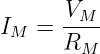
A real voltmeter has a finite input resistance RM. It draws approximately
for DC operation. A real ammeter has nonzero internal resistance and introduces an ammeter
burden voltage, often written
where RA is the effective current-path resistance. DMM specifications may instead give a
maximum burden per measurement range. In high-resistance or low-voltage circuits, both loading
mechanisms may matter.
5 Experiment 1: Ohm’s law from independently measured data
5.1 Prediction
Connect a resistor R to an adjustable DC source. If it is approximately ohmic over the tested
range,
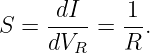
Thus, a plot of measured current I against measured resistor voltage V R should be linear, with
slope
The slope-inferred resistance is
This is better than comparing current with the bench supply’s displayed voltage, since an
ammeter burden or supply-lead drop may make that displayed voltage different from
V R.
5.2 Construction and measurement
- With power off, measure the actual value of a nominal 470 Ω resistor and record the
DMM range.
- Wire the resistor in series with the DMM current input. Connect a second DMM
across the resistor for voltage. With one DMM, disable the source before reconnecting
the meter, then repeat the setting to obtain voltage. Since reconnecting changes the
current-path burden, a second meter or a separately measured sense resistor gives a
more consistent two-quantity measurement.
- Set the current limit conservatively and raise the supply through approximately 1, 2,
3, 4, and 5 V.
- Record actual V R and I at each setting, not only the source display.
- Plot I against V R. Fit a straight line and compare 1∕S with the independently
measured resistor value.
- Reverse the resistor connections. Repeat one point. For a simple resistor, the measured
positive V∕I ratio should not depend on orientation.
A resistor measured at 470 Ω and carrying 10.0 mA should have a voltage of
This number is an illustrative prediction, not a supplied experimental result.
5.3 Inference and perturbation
Check whether the fitted intercept is consistent with zero within experimental resolution. A
significant intercept may indicate offset, an inappropriate measurement range, or recording error.
Repeat with a different resistance. An Ohm’s-law experiment is complete only after the changed
component has produced the expected change in slope.
6 Experiment 2: an unloaded and loaded voltage divider
6.1 Prediction without a meter
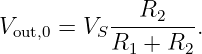
Two resistors R1 and R2 connected in series across a DC source V S form a voltage
divider. Taking the bottom node as reference, the output without a measurement load
is
For R1 = R2, the output is V S∕2. But an attached voltmeter provides another path from the
output node to the reference node.
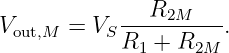
6.2 Loaded prediction
With input resistance RM, the lower leg becomes
Therefore,
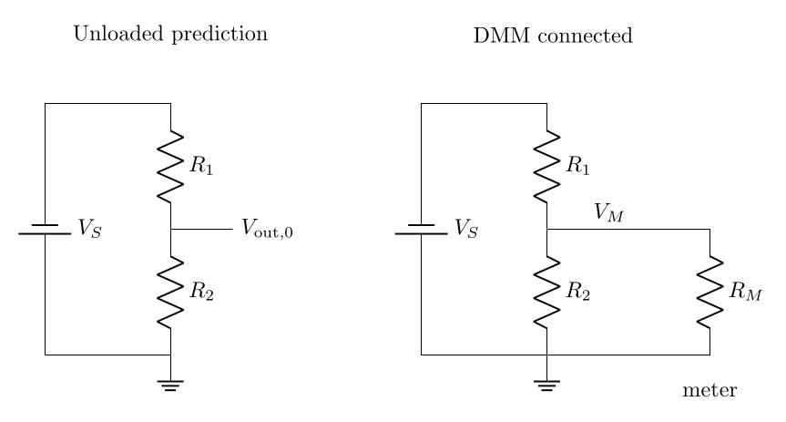
Figure 2. A divider without the meter (left) and with the meter’s finite input resistance in parallel
with the lower resistor (right). The measurement can alter the voltage it is intended to report.
The divider can also be described by its Thevenin parameters:
| V th | = V S , | (15)
|
| Rth | =  . | (16) |
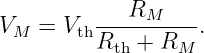
The voltage observed with the meter is
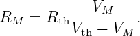
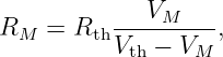
We can solve this expression for the unknown meter input resistance:
This inference becomes sensitive to measurement errors if the loading is too small. Choose a
divider whose Rth is a substantial fraction of RM while keeping the DMM input within its specified
measurement range.
6.3 Procedure
- Assemble a divider with R1 = R2 = 10 kΩ and V S ≃ 5 V. Record the actual values
and measured V S.
- Measure the output and compare with the unloaded prediction.
- Replace both resistors with values near 2.2 MΩ. Keep the supply voltage unchanged
and repeat.
- Calculate RM using measured resistances and voltages.
- Change the DMM range, if possible, and repeat. Do not assume that the input
resistance is constant on every range or in a high-impedance mode.
6.4 Worked illustrative estimate
Let V S = 5.00 V, R1 = R2 = 2.20 MΩ, and RM = 10.0 MΩ. Then
The measured-node prediction is
The meter depresses the output by approximately 0.248 V. This is nearly 10% of the unloaded
value, even when the DMM behaves perfectly according to its specification.
7 Thevenin model: an experimentally inferred source
A Thevenin equivalent is a two-terminal model with an ideal open-circuit voltage V th in series with
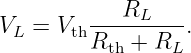
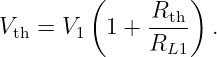
resistance Rth. For a resistive load RL, the terminal voltage is
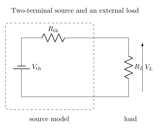
Figure 3. Thevenin source model. The load sees a voltage reduced by the series source resistance.
Measurements using different loads permit both source parameters to be inferred.
The model is an experimentally useful two-terminal description for a linear network at DC.
For an AC generator, Rth is a practical approximation to the output impedance over a
specified frequency range. Do not assume the impedance stays purely resistive at every
frequency.
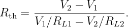
With two load values (RL1,RL2) and observed terminal voltages (V 1,V 2), we have
| V 1 | = V th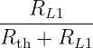 , | (22)
|
| V 2 | = V th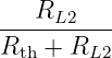 . | (23) |
Equating the resulting expressions for V th gives
The source voltage can then be recovered from either load:
The two-load formula is especially helpful when a true open-circuit measurement would be
distorted by the measuring instrument.
8 Experiment 3: measure a function generator’s source resistance
8.1 Prediction
A common laboratory generator has a nominal 50 Ω output impedance. This is a typical
instrument design, not a universal specification. The voltage shown on its display may be
calibrated for a specified load (usually 50 Ω or high impedance). Accordingly, the displayed
amplitude is not necessarily the open-circuit terminal amplitude.
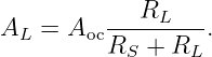
Let the actual open-circuit sine-wave amplitude be Aoc. For a resistive load,
Measure the same amplitude convention, preferably peak-to-peak voltage V pp, in all runs. Do not
mix peak, RMS, and peak-to-peak amplitudes. For a zero-offset sine wave,
8.2 Procedure: optional oscilloscope track
- Choose a sine wave near 1 kHz. Start with a small amplitude, such as about 1 Vpp when
the display is configured for high-impedance loading. Keep output offset at zero.
- Inspect the generator’s amplitude-load setting and document it. Connect the scope
ground to the generator’s signal return only.
- Measure the output amplitude with a high-impedance 10× probe and no added load.
This is an approximation to the open-circuit amplitude.
- Attach a measured 1 kΩ resistor from signal to return and record its terminal V pp.
- Replace the load with a measured 100 Ω resistor and record V pp again. Verify that the
generator is rated to drive it.
- Infer RS using both the open-circuit approximation and the two-load formula. Compare
the results.
- Repeat at a second, moderate frequency to test whether the inferred resistance is
approximately stable.
If RS = 50 Ω and the open-circuit amplitude is 1.00 Vpp, then the predicted amplitudes
are
| A1k | = 1.00 ≃ 0.952 Vpp, | (28)
|
| A100 | = 1.00 ≃ 0.667 Vpp. | (29) |
These are examples, not substitute data. The measured resistor values and scope readouts belong
in the lab record.
9 Experiment 4: oscilloscope probe loading
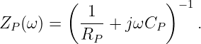
A probe does not merely transport a voltage to the oscilloscope. Its input is reasonably modeled,
over a restricted frequency range, by an effective resistance RP in parallel with an effective
capacitance CP :
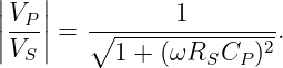
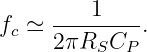
The source resistance RS and probe capacitance create a low-pass effect. If resistive input loading
is negligible,
Its approximate corner frequency is
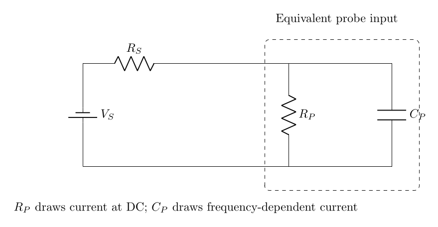
Figure 4. A source with nonzero output resistance driving the oscilloscope input. The probe
resistance and capacitance both load the measurement point. A 10× probe usually presents less
capacitance than direct 1× probing.
A common bench scope input is about 1 MΩ with appreciable parasitic capacitance;
a suitable 10× passive probe may present about 10 MΩ and a much smaller effective
capacitance. The actual values depend on the scope, probe, and attenuation switch. An
uncompensated passive probe can distort square-wave edges even when its DC attenuation is
correct.
9.1 Procedure
- Connect the generator through a measured 100 kΩ series resistor to a scope input. Use
a small sine wave.
- Begin at about 1 kHz. Compare source-side and measurement-node amplitudes when
a second scope channel is available.
- Repeat around 10, 20, and 50 kHz, keeping the source amplitude fixed.
- Compare the 1× connection with a correctly configured 10× probe. Match the probe
attenuation setting in the scope.
- Compare measurements with the model using the manufacturer’s approximate RP and
CP . Note that cable capacitance and compensating networks can modify the simple
model.
Do not use a long, unmatched loose wire as an assumed equivalent to a calibrated scope probe. A
10× probe must be compensated according to the scope manufacturer’s instructions before
interpreting edge shape.
10 Experiment 5: RC charging and discharging
10.1 Prediction from charge continuity
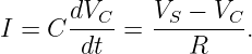
For a resistor R in series with a capacitor C, charge continuity and Ohm’s law give
For a step from zero to constant V 0 with V C(0) = 0,
For discharge through R from initial voltage V 0,
The RC time constant is
At t = τ, the ideal charging response reaches 1 − e−1 ≃ 0.632 of its final voltage, while the
discharging response falls to e−1 ≃ 0.368 of its initial value.
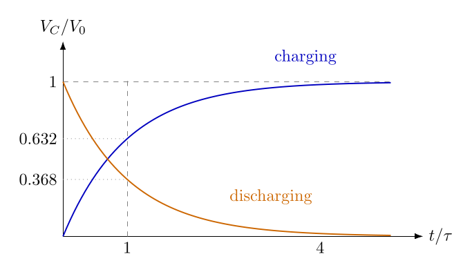
Figure 5. RC step-response geometry. The charging curve reaches 63.2% of its final value after one
time constant; the discharging curve falls to 36.8% of its starting value.
10.2 Track A: slow response with a DMM
- Measure a 100 kΩ resistor and a nominal 47 μF capacitor. Check polarity for an
electrolytic type.
- Connect R and C as a low-voltage series charging circuit. Connect the DMM across
the capacitor.
- Predict τ ≃ 4.7 s using nominal values.
- Apply about 5 V and record V C at t = 0, 2, 5, 10, 15, and 20 s or at comparable
intervals.
- Disable and disconnect the source, discharge through the resistor, and record the
voltage-decay curve. Do not directly short the capacitor.
- Estimate τ from the 63.2% or 36.8% time, noting the DMM update rate and manual
timing uncertainty.
For this arrangement, the DMM’s finite input resistance is in parallel with the capacitor.
It can shift the steady-state voltage and the inferred transient time constant. Check
whether RM is sufficiently large compared with R or incorporate it into the circuit
model.
10.3 Track B: function generator and oscilloscope
- Use a resistor near 10 kΩ and a capacitor near 100 nF, with predicted τ ≃ 1.0 ms.
- Apply a low-frequency square wave, about 20 to 25 Hz, with a safe amplitude and offset
that keep the capacitor within its ratings.
- Probe the capacitor using 10× mode. Record the voltage just after the edge and several
points through the transition.
- Determine τ from the 63.2% rise, the 36.8% decay, or from t90 − t10 ≃ 2.197τ for an
ideal rising exponential.
- Replace R with approximately twice its original value. Check whether the observed
time constant approximately doubles.
A function generator contributes additional source resistance. If its output resistance is relevant to
the experiment, replace R in the simple model by R + RS, after verifying the topology and
loading.
11 Experiment 6: understand oscilloscope ground
On a typical earth-grounded two-channel bench oscilloscope, the ground clips on both
channels are electrically common. They are also normally connected to the protective-earth
conductor through the instrument chassis. The probe tip measures its voltage relative to this
ground.
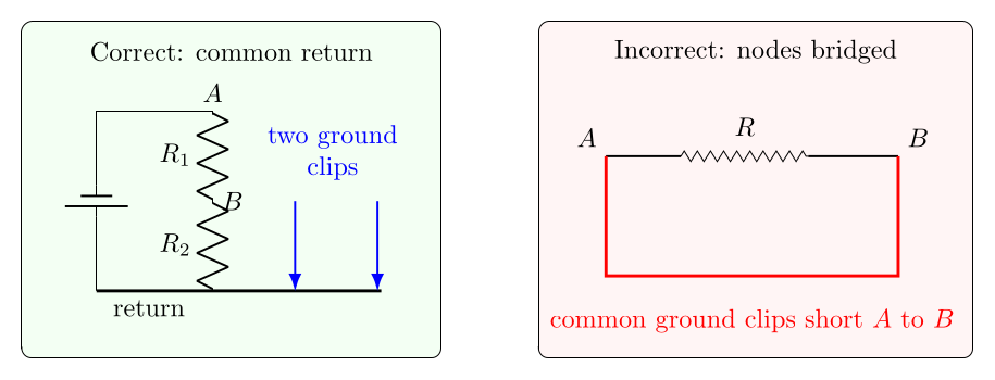
Figure 6. Left: two scope channels referenced to the same circuit return. Right: two ground clips
attached to different nodes can join those nodes electrically, causing an unintended short. Never
defeat the scope’s protective earth.
For an ordinary low-voltage series RC circuit, connect both scope ground clips to the circuit
return. Connect channel tips to the source and capacitor nodes. The difference between channels
may be computed using a verified scope math function, such as V R = V CH1 −V CH2, provided both
channels share the same reference and their settings match. This does not require connecting a
ground clip to the resistor’s upper node.
11.1 Safe demonstration
- With all outputs disabled, use a continuity function to check whether the scope channel
ground shells are common. Verify behavior with the instrument manual.
- Build a divider or RC circuit using only the approved low-voltage source and a single
designated return node.
- Attach both probe grounds to that return node.
- Observe the separate node voltages and, if available, their difference using the scope
math channel.
- Sketch a proposed but unconnected ground lead attached to an intermediate node.
Identify which component would be bypassed. Do not make the short to demonstrate
it physically.
Battery-operated isolated scopes and differential probes can have different reference behavior.
Isolation must be verified from their manuals; it must not be assumed from appearance or
portability.
12 Quantifying the uncertainty
An experimental value should be reported with at least an estimated measurement uncertainty and
a description of significant systematic effects. For a derived resistance R = V∕I, independent small
uncertainties give
If the same instrument introduces correlated errors, this expression is only an approximation.
Manufacturer accuracy statements can include a percent of reading plus a number of counts.
Instrument resolution is not identical to accuracy.
For a capacitance inferred from τ = RC,
so, for independent uncertainties,
For the inferred DMM input resistance,
errors become magnified when V M is nearly equal to V th. A divider selected to make loading
visible therefore produces a more stable inference than one with negligible observed
loading.
Each experiment should report
- the measured component values and instrument model or range;
- the theory prediction using those values;
- observed voltages, currents, or transient times;
- an instrument-loading estimate;
- at least one deliberate change to the apparatus;
- and an explanation of the dominant uncertainty.
13 Data processing and lab deliverables
The accompanying package includes blank CSV worksheets for experiments 1 through 5, an
example prediction worksheet, and a small Python analysis script. The example values in the
prediction worksheet are synthetic illustrations, not measured observations. Keep your raw data
separate from derived results.
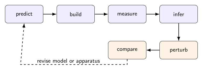
Figure 7. The EDL workflow distinguishes a theoretical prediction, the circuit that is actually
built, the instrument reading, and an inferred physical parameter. A deliberate perturbation
checks whether the model has predictive value.
For each experiment, include a circuit sketch, a table of raw measurements, one graph
with axes and units, at least one fitted or inferred parameter, and a concise physical
interpretation. Include an explanation when the measured result is inconsistent with the ideal
model.
14 Concept questions and experimental challenges
- A voltmeter reads 2.25 V across a nominally equal high-resistance divider connected
to a 5.00 V source. Why is that not necessarily evidence that either divider resistor is
defective?
- Why does measuring the voltage at the DMM terminals matter in an Ohm’s-law
experiment using a series ammeter?
- A generator gives about twice the peak-to-peak voltage into a high-impedance input
as into a 50 Ω termination. What source model does this suggest, and what limitations
remain?
- A passive scope probe shows a rounded square-wave edge. Give two possible physical
causes unrelated to the device under test.
- Why can connecting channel 1 ground to one RC node and channel 2 ground to a
different RC node alter the circuit even before measuring anything?
- An RC transient is measured with a slow DMM and then with a scope. What sources
of uncertainty dominate in the two cases?
- In the divider experiment, propose two changes that would reduce loading, and explain
the tradeoff between power consumption and measurement accuracy.
15 Answers and physical interpretation
- The DMM has a finite input resistance in parallel with the divider’s lower resistor; this
changes its output. Use a loaded-divider calculation.
- The ammeter has finite burden and the source leads have nonzero resistance; the
resistor voltage is the quantity that belongs in V R = IR.
- A source near 50 Ω in series with an ideal voltage may explain the half-amplitude
observation. Display loading settings and frequency-dependent impedance still need
checking.
- Probe capacitance and incorrect passive-probe compensation can round or distort
edges, in addition to the circuit’s genuine bandwidth limitation.
- On a common-ground scope, the ground clips electrically join the nodes and may bypass
a component or short the source.
- Manual timing and display update speed often dominate the slow experiment.
Probe loading, trigger placement, bandwidth, and sampling can matter in the scope
experiment.
- Reduce divider resistance or use a higher-impedance measurement system. Lower
divider resistance reduces fractional meter loading but increases supply current and
resistor dissipation.
16 Connection to the rest of electrodynamics
The instrument is part of the electromagnetic system, not an invisible observer. This practical fact
links the circuit experiments to the later field description. Current is transported charge, terminal
voltage is a potential difference, a capacitor stores electric-field energy, and source impedance
controls energy transfer. As measurement frequency rises, capacitance, inductance, spatial
distribution, and propagation increasingly matter. The simple lumped-element models used here
will be tested and refined in later EDL entries.
The next laboratory, EDL02, begins electrostatics and charge-induction experiments. EDL01
provides the measurement discipline needed to distinguish physical electric-field effects from
detector and instrument artifacts.
17 References
- PhysicsLibrary, EDL00, Home Electrodynamics Laboratory: Roadmap, Bench Setup,
Measurement Practice, and Griffiths Companion.
- D. J. Griffiths, Introduction to Electrodynamics, 5th ed., Cambridge University Press.
Unofficial experimental companion.
- Relevant operating manuals and input/output specifications for the DMM, oscilloscope,
probes, DC supply, and function generator actually used.