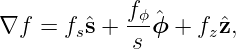
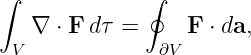
ED03: Gradient, Divergence, Curl, and the Geometry of Differential Operators
The electrical and magnetic fields in ED01 are not just vectors. They are vector fields: their
magnitudes and directions may change from one point to another. ED02 developed the geometry
needed to describe those changes, including local basis vectors, physical lengths, surface elements,
and volume elements. We now build the three central operations of vector calculus from that
geometry.
- The gradient of a scalar field describes how rapidly that scalar changes, and in which
direction it increases most strongly.
- The divergence of a vector field measures the net outward flux per unit volume as the
volume shrinks to a point.
- The curl of a vector field measures its local oriented circulation per unit area as the
loop shrinks to a point.
The goal is to understand why the familiar coordinate formulas have their particular terms. In
particular, the factors 1∕s, 1∕r2, and 1∕(r sin 𝜃) in cylindrical and spherical coordinates are
geometric consequences of the scale factors derived in ED02; they are not arbitrary algebraic
decorations.
This article develops the local differential operators and previews their role in Electromagnetism.
Full proofs of Gauss’s and Stokes’ integral theorems are reserved for ED04.
1 Three questions to ask of a field
Suppose a scalar field is
We can ask how much V changes if we take a small step. The answer is encoded by ∇V , the
gradient.
Suppose instead we have a vector field
We can ask whether more of the field leaves a tiny volume than enters it. This is divergence. We
can also ask whether the field tends to circulate around a tiny oriented loop. This is
curl.
These are different questions. A field can have zero divergence but nonzero curl, nonzero
divergence but zero curl, or both zero in some region.
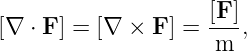
For a field with physical units [F], the divergence and curl have units
while the gradient of a scalar f has units [f]∕m.
2 The gradient begins with a one-dimensional derivative
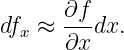
For a function f(x), the derivative is the limiting change per unit distance,
For a function of three variables, a small change in x contributes
Changes in y and z contribute similarly. Adding all three first-order contributions gives the total
differential,
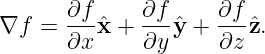
The differential displacement is
Equation (6) has the form of a dot product. Define
Then the compact differential statement is
Equation (9) gives the gradient its geometric meaning. It is the vector whose dot product with a
small displacement gives the first-order change in the scalar field.
3 Directional derivatives and the steepest direction
Consider a displacement along a unit direction u,
Substitute into Equation (9):
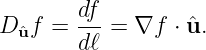
Dividing by dℓ and taking the limit defines the directional derivative,
Let α be the angle between ∇f and u. Then
Because cos α ≤ 1, the largest possible increase per unit distance is |∇f|, attained in the direction
of ∇f. The fastest decrease occurs in the opposite direction.
If a displacement is tangent to a surface on which f is constant, then df = 0, and
Thus the gradient is Normal to a level surface wherever the gradient is nonzero.
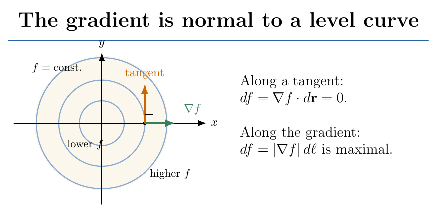
Figure 1. The gradient of a scalar field points normal to its level curves and toward increasing
values. A tangent displacement along a level curve produces no first-order change in the scalar.
4 Worked example: a quadratic scalar field
Let
Compute the three partial derivatives:
Therefore
At (1,−1, 1),
Its magnitude is
To find the rate of change along the +y direction, choose u = y:
So the function decreases by approximately 4 dℓ for a short positive y displacement at that
point.
5 Gradient and electric potential
In electrostatics, the electric field is related to scalar electric potential by
The minus sign means that the electric field points in the direction of most rapid decrease of
electric potential. The reason can be stated through the work done on a positive test charge
q:
Equipotential curves are therefore everywhere perpendicular to the electrostatic field where E≠0.
An instrument may measure values of V at many points, and the gradient allows us to infer E
from those measurements.
The relation E = −∇V is for electrostatic fields. In time-dependent electrodynamics, a
vector-potential term is also required, as ED01 previewed.
6 Flux as the starting point for divergence
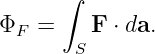
For a surface with oriented area element da, define the flux of a vector field as
This dot product selects the part of F normal to the surface. A component tangent to the surface
does not contribute to flux through it.
To understand divergence locally, surround a point by a small closed volume ΔV . Define the net
outward flux divided by the volume, then let the region shrink to the point:
The limit assumes the field is sufficiently smooth at the point. A positive value means net outward
flux per unit volume; a negative value means net inward flux. Neither case requires fluid to be
physically created or destroyed: divergence is a property of the vector field, and its physical
interpretation depends on what F represents.
7 Deriving Cartesian divergence from a small box
Take a rectangular box of edge lengths Δx, Δy, and Δz, centered at (x,y,z). Its volume
is
Consider only the two faces perpendicular to x. The outward normal of the right face is +x; the
left-face normal is −x.
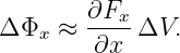
For a sufficiently small box, the combined outward flux through those two faces is
| ΔΦx ≈ | Fx 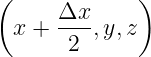 ΔyΔz | (26)
|
| − Fx 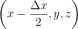 ΔyΔz. | (27) |
Divide and multiply by Δx:
| ΔΦx ≈ |  | (28)
|
| × ΔxΔyΔz. | (29) |
The partial derivative appears when Δx → 0:
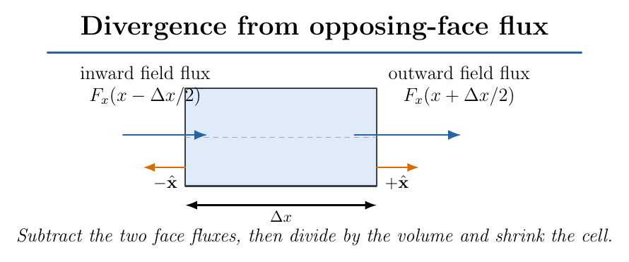
Figure 2. The outward flux through opposing faces is a difference, not a sum of unsigned arrow
magnitudes. A spatial increase in the outward x component produces positive net flux through
the small volume.
Repeat the same argument for the faces perpendicular to y and z:
| ΔΦy | ≈ ΔV, | (31)
|
| ΔΦz | ≈ ΔV. | (32) |
Adding the six-face fluxes, dividing by ΔV , and taking the limit gives
Notice that the derivative of Fx with respect to x appears because flux through x-normal faces
is being compared. Divergence does not sum all nine spatial derivatives of a vector
field.
8 Divergence examples and an important caution
Consider
Then
There is positive outward flux per unit volume at every point.
A uniform vector field,
has zero divergence because the same flux that enters one side of a small box leaves the opposite
side.
Do not interpret a field that points outward as necessarily having positive divergence everywhere.
For example, the field
points outward for C > 0, but has zero divergence at every point where r > 0. Its singularity at
r = 0 needs separate treatment, introduced later in ED05 and ED09.
9 Circulation as the starting point for curl
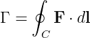
The line integral
measures the field’s component along a closed oriented loop. The direction around the loop is
chosen consistently with its normal by the right-hand rule.
To measure local circulation, shrink a loop with oriented normal n toward a point and divide by its
enclosed area:
The components of curl are obtained by choosing infinitesimal loops whose normals are the
coordinate basis directions. A positive normal component means positive circulation when viewed
in the corresponding right-hand orientation.
10 Deriving the Cartesian z component of curl
Take a counterclockwise rectangular loop in the xy plane, with sides Δx and Δy. Its oriented
normal is +z.
For the bottom edge, the displacement is along +x:
On the right edge, the displacement is along +y:
The top edge runs along −x:
The left edge runs along −y:
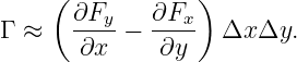
Add the four contributions and group them:
| Γ ≈ |  Δy | (44)
|
| − Δx. | (45) |
Take the first-order Taylor approximations,
| Fy(x + Δx,y) − Fy(x,y) | ≈ Δx, | (46)
|
| Fx(x,y + Δy) − Fx(x,y) | ≈ Δy. | (47) |
Therefore
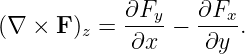
Divide by the loop area and shrink the loop:
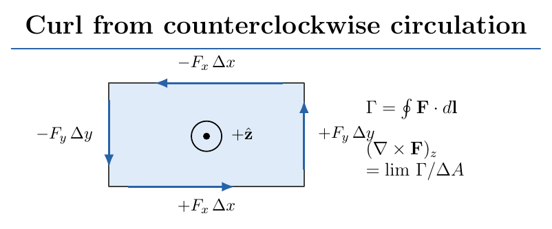
Figure 3. Counterclockwise circulation around a shrinking xy loop defines the +z component of
curl. The top and left edge contributions have minus signs because those edges are traversed in
negative coordinate directions.
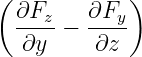
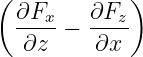
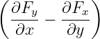
Repeating the procedure with loops normal to the x and y axes yields the full Cartesian
expression:
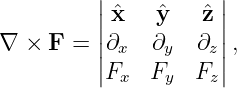
An equivalent memory aid is the formal determinant,
but the shrinking-loop derivation is the geometric meaning behind that notation.
11 Curl, rotation, and the factor of two
Consider a rigidly rotating velocity field in the xy plane,
where Ω is a constant angular speed about +z.
Compute its curl:
| (∇× v)z | =  −  | (53)
|
| = Ω − (−Ω) = 2Ω. | (54) |
Hence
The curl is twice the local rigid-body angular velocity for this special velocity field. In fluid
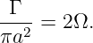
mechanics curl of velocity is called vorticity. For a circular path of radius a, the line integral gives
the same answer:
The circulation per unit area is
Curl measures local circulation, not necessarily whether the field lines visually look bent. A curved
pattern of field lines by itself does not establish nonzero curl.
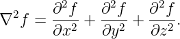
12 The Laplacian is divergence of a gradient
Once gradient and divergence are defined, a new scalar differential operator follows
naturally:
Substitute Equation (8) into the Cartesian divergence formula:
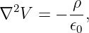
The Laplacian combines the spatial change of the gradient in all three directions. In electrostatics
it appears in Poisson’s equation,
and in charge-free electrostatic regions as Laplace’s equation,
We are previewing those equations; ED09 onward will derive and solve their physical
boundary-value problems.
13 Why ED02’s scale factors are the missing geometry
Let q1,q2,q3 be orthogonal coordinates, with position vector
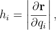
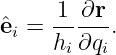
ED02 defined the scale factors by
and the local unit basis vectors by
An infinitesimal displacement is
The small cell volume is
A face normal to e1 has area
with cyclic expressions for the other faces.
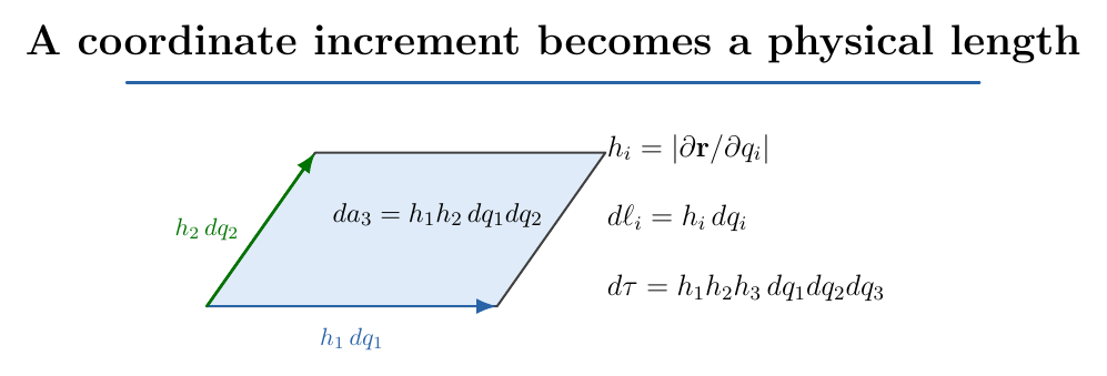
Figure 4. A coordinate increment dqi is not generally a physical length. Its physical edge is hi dqi.
The product of two physical edges gives a face area, and the product of three gives a volume.
For the derivations below, we assume a smooth right-handed orthogonal coordinate basis away
from coordinate singularities.
14 General gradient in orthogonal coordinates
The scalar differential is coordinate independent:
Write the unknown gradient as
The defining relation is again
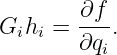
Using Equation (65) and orthonormality,
Compare coefficients of each independent coordinate increment:
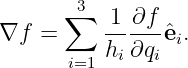
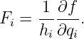
Therefore
The factor 1∕hi is simply the conversion from a change per unit coordinate to a change per unit
physical length.
15 General divergence from a curvilinear flux balance
Write the vector field in the local orthonormal basis,
Examine the two faces normal to e1. To first order, the outward flux difference is
Notice the derivative of both F1 and the face-area factor h2h3. When the coordinate geometry
changes with position, an opposing face can have a different area even if the component F1 is
numerically unchanged.
Add the other two pairs of faces,
| dΦ2 | ≈ (h3h1F2) dq1dq2dq3, | (76)
|
| dΦ3 | ≈ (h1h2F3) dq1dq2dq3. | (77) |
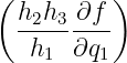
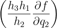
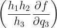
Divide their sum by the volume in Equation (66). The general divergence is
∇⋅ F =   |  (h2h3F1) | |
|
| +  (h3h1F2) | |
|
| +  (h1h2F3) ![]](https://images.physicslibrary.org/cache/objects/1584/make4ht/GradientDivergenceCurlAndTheGeometryOfDifferentialOperators83x.png) . | (78) |
This is the single formula from which the familiar Cartesian, cylindrical, and spherical divergence
expressions follow.
16 General curl from a curvilinear loop
Take a small loop whose sides follow the q1 and q2 coordinate curves, oriented so that the normal
points along +e3.
The physical edge along q1 is h1dq1, and the edge along q2 is h2dq2. A first-order circulation
balance gives
| dΓ3 ≈ |  dq1dq2 | (79)
|
| − dq1dq2. | (80) |
The physical area is
Divide circulation by area and shrink the loop:
Cyclic permutations supply the other components:
| (∇× F)1 | =  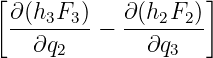 , | (83)
|
| (∇× F)2 | =  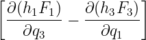 . | (84) |
These formulas automatically account for physical edge lengths and rotating basis directions. They
should be used with components referred to the local orthonormal unit vectors, not unnormalized
coordinate tangent vectors.
17 General scalar Laplacian
Apply the general divergence formula to F = ∇f.
The gradient components are
Substitution yields
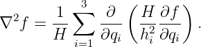
Equivalently, if H = h1h2h3,
This is the scalar Laplacian. A vector Laplacian is a different, vector-valued operation and must
not be obtained by blindly applying the scalar expression to curvilinear components.
18 Specialization to Cartesian coordinates
In Cartesian coordinates,
Every scale factor equals one, so the general formulas immediately reduce to
and Equation (50) for curl. The Laplacian is Equation (59).
Cartesian formulas look simpler partly because the Cartesian basis directions and coordinate areas
do not change from place to place.
19 Cylindrical coordinates: derive the gradient
ED02 used
with scale factors
Insert these into Equation (73):
The azimuthal derivative has the factor 1∕s because the physical distance for an angle dϕ is sdϕ.
The same change of f over a longer arc length corresponds to a smaller physical gradient
component.
For example, if
then
Therefore
20 Cylindrical coordinates: derive the divergence
For (hs,hϕ,hz) = (1,s, 1), the total scale factor product is
The face-area products in Equation (78) are
Substitute carefully:
∇⋅ F =   |  (sFs) +  | |
|
| +  (sFz) ![]](https://images.physicslibrary.org/cache/objects/1584/make4ht/GradientDivergenceCurlAndTheGeometryOfDifferentialOperators119x.png) . | (99) |
Since s does not depend on z,
To understand the first term geometrically, consider a thin cylindrical shell. Its curved inner and
outer faces have circumferences proportional to s. The larger face can carry more flux even if the
radial component Fs is unchanged.
For F = Cs with constant C,
Thus a field of constant radial magnitude in cylindrical coordinates does not have zero divergence.
The increasing circumference matters.
21 Cylindrical coordinates: derive the curl
Use Equations (83) through (82) with (hs,hϕ,hz) = (1,s, 1).
For the radial component,
| (∇× F)s | =  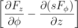 | (102)
|
| =   −  . | (103) |
For the azimuthal component,
| (∇× F)ϕ | =  −  . | (104) |
For the axial component,
| (∇× F)z | =  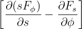 . | (105) |
Putting these components together,
The term ∂(sFϕ)∕∂s contains the geometry of circular paths. It should not be replaced by
s∂Fϕ∕∂s unless the derivative of s is also included.
22 Cylindrical scalar Laplacian
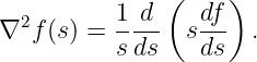
The scalar Laplacian follows from either the general formula or ∇⋅ (∇f):
If a scalar is independent of ϕ and z, only the radial term survives:
This radial form will be useful for long-wire, cylindrical Conductor, and coaxial-electrode
problems.
23 Spherical coordinates and their scale factors
ED02 used
where 𝜃 is the polar angle measured from +z and ϕ is the azimuth about z.
The scale factors are
Thus
The factor r sin 𝜃 is the physical radius of a circle of latitude. In particular, the azimuthal distance
r sin 𝜃 dϕ shrinks near the poles, even if dϕ is unchanged.
24 Spherical gradient
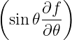
Insert Equation (110) into the general gradient:
The three terms each mean a change in f per unit physical distance along one of the local
orthogonal directions.
As a check, let f = r. Then
Increasing the radial coordinate by one meter increases the scalar distance r by one meter. Motion
tangent to a sphere does not change r to first order.
25 Spherical divergence and its geometric interpretation
The three face-area products are
Substitute into the general divergence and simplify:
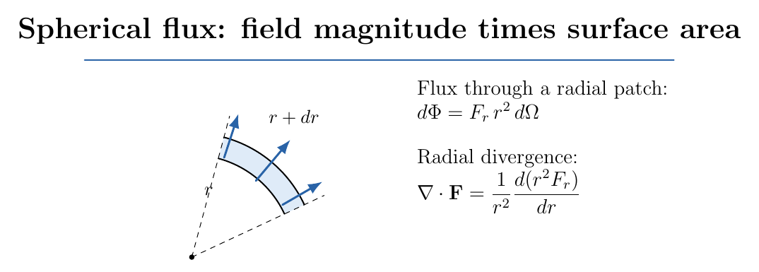
Figure 5. The outward flux through a spherical surface depends on both field magnitude Fr and
the expanding surface area proportional to r2. The radial divergence term differentiates their
product r2Fr.
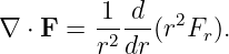
For a purely radial field F = Fr(r)r, all angular terms vanish:
Two important checks follow.
If Fr = C,
If instead Fr = C∕r2,
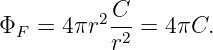
For the inverse-square field, the growing spherical area exactly compensates for the decreasing
radial magnitude. Its flux through any sphere centered at the origin is
This zero-divergence calculation is valid away from the origin. The singular point itself must not be
discarded. Its treatment requires the Dirac delta distribution, a subject developed later in the ED
sequence.
26 Spherical curl
Use the general curl equations with (hr,h𝜃,hϕ) = (1,r,r sin 𝜃).
For the radial component,
| (∇× F)r | =  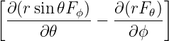 | (121)
|
| =  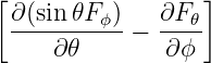 . | (122) |
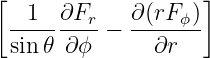
For the polar component,
| (∇× F)𝜃 | =  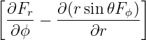 | (123)
|
| =   . | (124) |
For the azimuthal component,
The spherical curl can therefore be assembled as
| ∇× F = | (∇× F)rr | |
|
| + (∇× F)𝜃𝜃 | |
|
| + (∇× F)ϕϕ. | (126) |
The component form above is often easier to read and apply than one very long three-component
equation.
27 Spherical scalar Laplacian
Apply divergence to the spherical gradient:
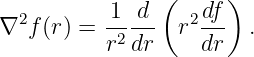
For a spherically symmetric scalar f(r),
This is the radial Laplacian used for the electrostatic potential of a spherically symmetric charge
distribution.
28 A common trap: constant components need not mean a uniform vector
In Cartesian coordinates, a spatially constant list of components describes a constant vector. In
curvilinear coordinates, basis vectors rotate with position.
For example, a uniform field in the +z direction is
ED02 gives the spherical decomposition
Therefore
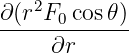
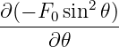
Use spherical divergence:
Evaluate each term:
The terms cancel, just as they must for a uniform Cartesian vector field.
If we had treated Fr alone as the whole field or omitted the angular basis contribution, we would
have obtained an incorrect divergence.
29 Two useful vector-calculus identities
For any sufficiently smooth scalar field f,
For example, its Cartesian z component is
| (∇×∇f)z | =   −   | (135)
|
| = fyx − fxy = 0, | (136) |
because mixed partial derivatives agree under the usual smoothness conditions.
Similarly, for a sufficiently smooth vector field F,
In Cartesian coordinates, substituting Equation (50) produces six mixed second derivatives that
cancel in pairs.
These are local identities. Statements about global potential functions require additional care with
domain topology and singularities. ED04 will connect local identities to closed-loop and
closed-surface integral laws.
30 Terminology: irrotational and solenoidal fields
A vector field is called irrotational in a region if
throughout that region.
A field is called solenoidal or divergence-free in a region if
throughout that region.
Those properties are distinct. A rigid-rotation velocity field is divergence-free but has nonzero curl.
An expanding radial field may have nonzero divergence but zero curl in a region where it is
smooth.
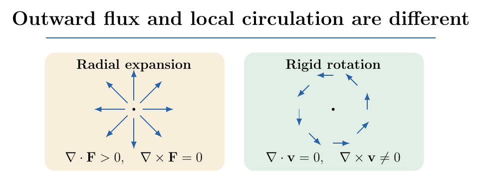
Figure 6. Two fields can have very different local differential properties. The planar radial field
shown has positive divergence and zero curl away from its center; rigid rotation has zero
divergence and curl directed along the rotation axis.
31 Worked electromagnetic example 1: potential mapping
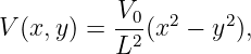
Suppose a two-dimensional electrostatic potential is modeled in a region by
where V 0 has units of volts and L has units of length.
Step 1: Differentiate the potential,
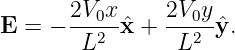
Step 2: Apply the electrostatic relation E = −∇V ,
Step 3: Compute the divergence,
| ∇⋅ E | = − +  | (143)
|
| = 0. | (144) |
Step 4: Compute the z component of curl,
| (∇× E)z | =  −  | (145)
|
| = 0 − 0 = 0. | (146) |
Thus this example is both divergence-free and curl-free in the modeled region. It is consistent
with the absence of local electrostatic charge there and with an electrostatic potential
field.
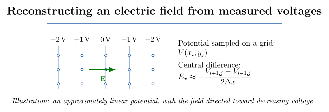
Figure 7. In a potential-mapping laboratory, a voltmeter samples the scalar V at neighboring
points. Differences of those samples estimate ∂V∕∂x and ∂V∕∂y, which determine the local
electric-field components.
A central-difference estimate from a grid is
and similarly
This is a practical example of the mathematical gradient acting on measured data. It is also a
reminder that a numerical estimate depends on probe spacing, noise, and measurement
resolution.
32 Worked electromagnetic example 2: charge density from divergence
Suppose a field within a region is
where α,β,γ are constants with units V∕m2.
Compute
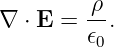
Gauss’s local electric law, previewed in ED01, is
Therefore the required charge density is
The result has correct units: 𝜖0 times V∕m2 has units C∕m3.
The curl of this field is zero, consistent with its representation by the electrostatic potential
33 Worked electromagnetic example 3: azimuthal magnetic field
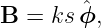
Consider a cylindrically symmetric field
where k is a constant with units T∕m.
The cylindrical divergence is zero because Bs = Bz = 0 and Bϕ is independent of ϕ:
The axial curl is
| (∇× B)z | =   | (156)
|
| =   | (157)
|
| = 2k. | (158) |
All other curl components vanish, so
For a steady magnetostatic field in vacuum, Ampere’s local law gives
Hence this field corresponds to uniform axial current density
This is a useful example because the azimuthal component must be differentiated together with the
geometric factor s.
34 Worked example 4: direct Cartesian computation
Let
Its divergence is
Compute the curl components,
| (∇× F)x | = x − x = 0, | (164)
|
| (∇× F)y | = y − y = 0, | (165)
|
| (∇× F)z | = z − z = 0. | (166) |
This field is the gradient of the scalar f = xyz:
The result therefore provides a direct check of the identity ∇×∇f = 0. Note, however, that the
divergence of a gradient is its Laplacian; the fact that it also vanishes here is a special property of
f = xyz, not a universal property of gradients.
35 Coordinate singularities and sources
Cylindrical formulas have factors 1∕s; spherical formulas have 1∕r, 1∕r2, and 1∕ sin 𝜃. These
expressions can be singular on coordinate axes or at the origin.
There are two distinct possibilities:
- The coordinate chart is degenerate even though the underlying physical field remains
smooth; a uniform Cartesian field expressed in spherical components is a common
example.
- The physical field is genuinely singular, as in the ideal electrostatic point-charge field
E ∝r∕r2 at the origin.
The coordinate formulas derived here apply directly only where the coordinate basis is defined and
the field is sufficiently differentiable. Distributions, point sources, line currents, and the role of the
domain will receive separate treatment in later articles.
36 How to choose the right operator
Before calculating, translate the physical question into a mathematical one.
- How does a scalar change with position? Compute ∇f. To get the rate along a specified
direction, compute ∇f ⋅u.
- Does a vector field have local net outward flux? Compute ∇⋅ F.
- Does it have local oriented circulation? Compute ∇× F.
- How does the gradient of a scalar spread or converge? Compute ∇2f = ∇⋅∇f.
Then choose coordinates that match the geometry. Do not substitute cylindrical or spherical
components into the Cartesian formulas without accounting for basis rotation and scale
factors.
37 Formula summary for Cartesian coordinates
For F = Fxx + Fyy + Fzz,
| ∇f | = fxx + fyy + fzz, | (168)
|
| ∇⋅ F | = Fx,x + Fy,y + Fz,z, | (169)
|
| ∇2f | = f
xx + fyy + fzz. | (170) |
Curl is given by Equation (50).
38 Formula summary for cylindrical coordinates
For (s,ϕ,z) with (hs,hϕ,hz) = (1,s, 1),
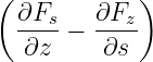
| (∇× F)s | =  ∂ϕFz − ∂zFϕ, | (173)
|
| (∇× F)ϕ | = ∂zFs − ∂sFz, | (174)
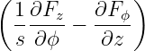
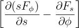
|
| (∇× F)z | =  [∂s(sFϕ) − ∂ϕFs], | (175) |
and
In these compressed formulas, subscripts s,ϕ,z on f indicate partial derivatives. Subscripts on the
vector components Fs,Fϕ,Fz identify basis components.
39 Formula summary for spherical coordinates
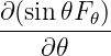
For (r,𝜃,ϕ) with (hr,h𝜃,hϕ) = (1,r,r sin 𝜃),
| ∇⋅ F = |  ∂r(r2F
r) | |
|
| +  ∂𝜃(sin 𝜃F𝜃) | |
|
| +  ∂ϕFϕ. | (178) |
The three spherical curl components are given explicitly in the spherical curl section, and the
scalar Laplacian is Equation (127). Keeping those formulas separated avoids a long expression that
is difficult to read and prone to rendering problems.
40 Common mistakes
- Thinking divergence is simply “arrows pointing outward.” It is a limit of net flux per
volume.
- Thinking curved field lines automatically imply nonzero curl. Curl is a local circulation
limit.
- Forgetting the right-hand orientation when computing circulation and curl.
- Treating ϕ and 𝜃 as lengths rather than angles with scale factors.
- Omitting the radial area factor r2 from spherical divergence.
- Omitting the factor s inside ∂s(sFϕ) in cylindrical curl.
- Treating a curvilinear basis as if its directions were fixed Cartesian basis vectors.
- Using the scalar Laplacian independently on vector components in a curved basis
without accounting for basis variation.
- Concluding that ∇⋅ (Cr∕r2) = 0 everywhere, including the undefined origin.
- Applying electrostatic E = −∇V to a time-dependent electromagnetic field without
the vector-potential term.
41 Practice exercises
- For f = x2y + z3, find ∇f and the directional derivative at (1, 2, 1) along (1, 1, 1)∕
 .
- Compute the divergence and curl of F = (x2,−2xy,z2).
- Derive the x component of Cartesian curl by applying the small-loop circulation
argument to a loop in the yz plane.
- Starting from (hs,hϕ,hz) = (1,s, 1), derive cylindrical divergence without quoting the
final formula.
- Show that the cylindrical field F = Cs∕s has zero divergence for s > 0.
- Use the cylindrical curl expression to compute curl of F = Ωsϕ.
- Starting from the spherical scale factors, derive the r component of spherical curl.
- Prove that ∇⋅ (Fr(r)r) = r−2d(r2F
r)∕dr for r > 0.
- Evaluate ∇2(rn) away from the origin for real n and identify the values of n for which
it vanishes.
- Show that a uniform Cartesian vector F0z has zero divergence using spherical
coordinates.
- For V (x,y) = V 0(x2 − y2)∕L2, compute E, its divergence, and its curl.
- Explain the physical difference between flux through a closed surface and circulation
around a closed curve.
42 Companion filebox resources
The following lightweight files are intended for uploading to the ED03 PhysicsLibrary filebox:
43 Summary and bridge to ED04
The gradient, divergence, and curl are local differential operators with complementary geometric
meanings:
Their curvilinear formulas are built from the same ED02 scale factors that convert coordinate
increments into physical lengths, areas, and volumes.
ED04 will establish the two major integral bridges:
and
Those theorems turn the local differential laws of Maxwell’s Equations into the integral forms used
throughout electrodynamics and laboratory measurements.
References
References
[1] D. J. Griffiths, Introduction to Electrodynamics, 5th ed., Cambridge University Press,
2023.
[2] E. M. Purcell and D. J. Morin, Electricity and Magnetism, 3rd ed., Cambridge
University Press, 2013.
[3] H. M. Schey, Div, Grad, Curl, and All That, 4th ed., W. W. Norton, 2005.
[4] M. L. Boas, Mathematical Methods in the Physical Sciences, 3rd ed., Wiley, 2006.
[5] G. B. Arfken, H. J. Weber, and F. E. Harris, Mathematical Methods for Physicists,
7th ed., Academic Press, 2013.




















































![]](https://images.physicslibrary.org/cache/objects/1584/make4ht/GradientDivergenceCurlAndTheGeometryOfDifferentialOperators101x.png)
















 +