ED06: Curvilinear Field Geometry, Scale Factors, and Vector Operators
Electrostatic and magnetic fields are geometrical objects. Their existence does not depend on
whether we label the same point by (x,y,z), (s,ϕ,z), or (r,𝜃,ϕ). Yet the formulas for divergence,
curl, and the Laplacian look different in different coordinates. Why?
The answer is that a coordinate increment is not necessarily a physical distance, and a local
basis vector need not point in the same direction at neighboring points. Both effects are
encoded in scale factors and in the geometry of infinitesimal line, area, and volume
elements.
ED02 developed the coordinates and their scale factors; ED03 derived the local operators; ED04
showed how flux and circulation become integral laws; ED05 examined idealized singular sources.
This article unifies those ideas by deriving the general orthogonal-curvilinear formulas, specializing
them to cylindrical and spherical geometries, and checking them against fields relevant to
Maxwell’s Equations.
1 One field, many coordinate descriptions
A vector is an object with magnitude and direction, independent of a coordinate chart. Relative to
the Cartesian basis, the vector is
At the same physical point, a cylindrical description is
The two sets of numbers generally differ, even though F is the same vector. Moreover, s and ϕ
rotate as the observation point moves around the axis.
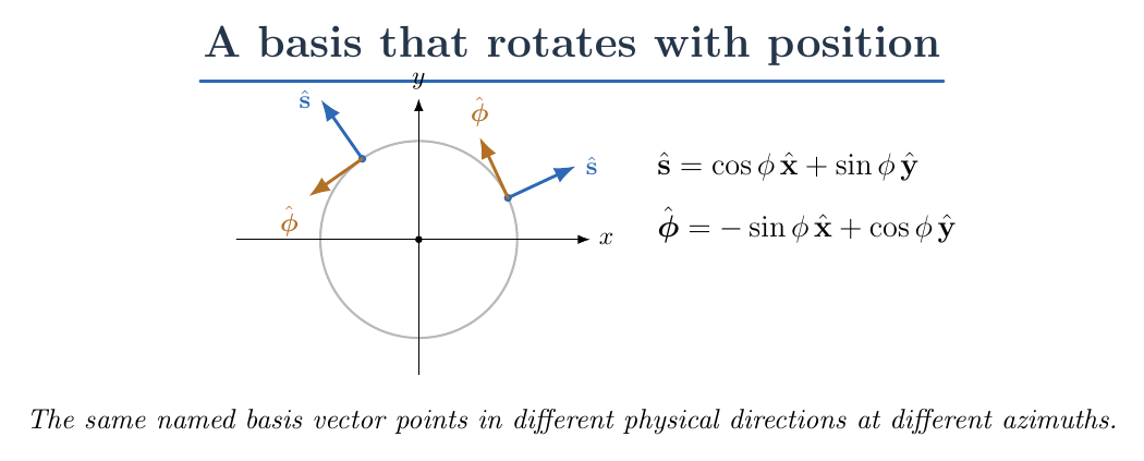
Figure 1. The cylindrical radial and azimuthal unit vectors change direction around the axis. A
field with constant cylindrical components need not be spatially uniform as a vector.
We use a right-handed orthonormal basis throughout. For spherical coordinates, 𝜃 means polar
angle measured down from +z, and ϕ means azimuth measured from +x toward +y. These
conventions matter when checking signs and cross products.
2 Constructing coordinates from the position map
Let a spatial position be described by three coordinates q1,q2,q3:
Changing qi while holding the other two coordinates fixed traces a coordinate curve. Its tangent
vector is
For an orthogonal coordinate system the three tangents are mutually perpendicular away from
coordinate singularities.
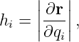
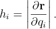
Define the scale factors
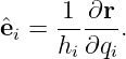
and the local unit vectors
Thus ∂r∕∂qi = hiei.
Physical meaning of hi
If only qi changes, then to first order
so the physical length of the small displacement is
In particular, an angle dϕ is dimensionless (measured in radians), but the arc length produced by
that angle has units of length. The scale factor performs the conversion.
3 The line element and its squared length
Differentiate Equation (3), allowing all coordinates to change:
| dr | =  dq1 +  dq2 +  dq3 | (9)
|
| = h1dq1e1 + h2dq2e2 + h3dq3e3. | (10) |
Dot this expression with itself. Orthogonality removes the six cross terms:
| ds2 = dr ⋅ dr = h
12dq
12 + h
22dq
22 + h
32dq
32. | | (11) |
The factors hi are consequently the square roots of the diagonal metric coefficients of an
orthogonal coordinate chart. Nothing about the physical Euclidean space has changed; only the
coordinate description has changed.
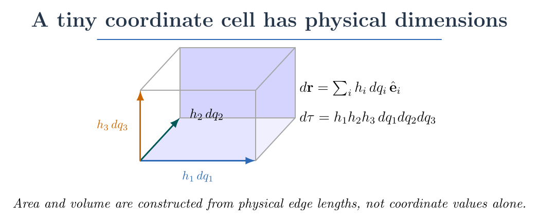
Figure 2. An infinitesimal orthogonal coordinate cell has physical edge lengths h1dq1, h2dq2, and
h3dq3. Its physical area and volume follow from those edges, not from raw coordinate increments.
4 Deriving the surface and volume elements
Hold q1 fixed. Two tangent edges of a small coordinate surface are
The oriented area vector follows from their cross product:
| da1 | = dl2 × dl3 | (13)
|
| = h2h3 dq2dq3e1. | (14) |
We have selected the positive orientation associated with the right-handed ordered basis. Reversing
the order of the tangent edges reverses the surface Normal. Similarly,
| da2 | = h3h1 dq3dq1e2, | (15)
|
| da3 | = h1h2 dq1dq2e3. | (16) |
Multiply one physical edge by the area normal to it:
For a nonsingular right-handed orthogonal chart, h1h2h3 is the positive coordinate Jacobian:
The absolute value |J| is used if a chart reverses orientation. These formulas are valid at regular
points where all required scale factors are nonzero.
5 Cylindrical scale factors, derived
Use cylindrical coordinates (s,ϕ,z) with
| x | = s cos ϕ, | (19)
|
| y | = s sin ϕ, | (20)
|
| z | = z. | (21) |
Write the Cartesian position vector:
Partial differentiation gives
 | = cos ϕx + sin ϕy = s, | (23)
|
 | = −s sin ϕx + s cos ϕy = sϕ, | (24)
|
 | = z. | (25) |
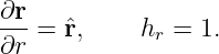
Consequently,
Substituting into Equations (10) and (17),
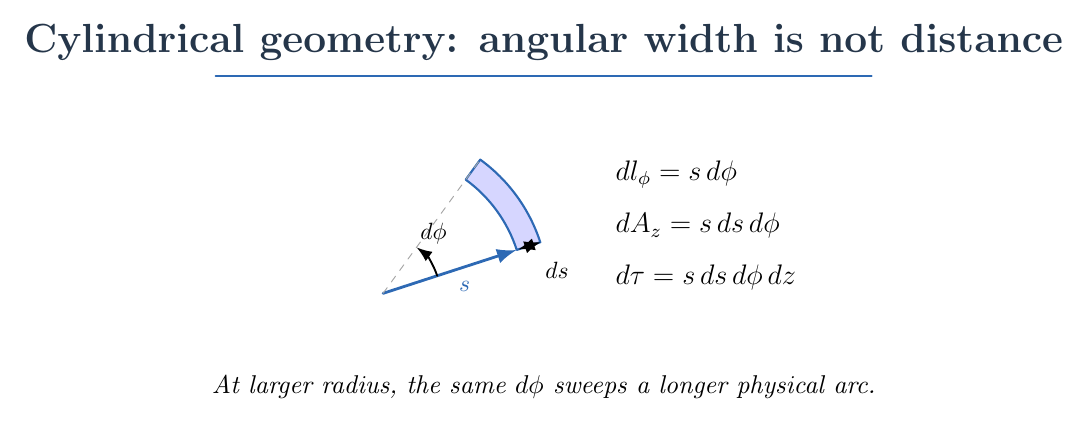
Figure 3. The physical angular width of an annular cylindrical wedge is sdϕ. A wedge at larger
radius is physically wider even when dϕ is unchanged.
The area of a cylindrical side at fixed s is sdϕdz. A horizontal face at fixed z has area sdsdϕ.
These are different because they lie in different coordinate surfaces.
6 Spherical scale factors and the latitude radius
In spherical coordinates, the position vector is
| r = | r sin 𝜃 cos ϕx + r sin 𝜃 sin ϕy | (29)
|
| + r cos 𝜃 z. | (30) |
Differentiate with respect to r:
Differentiate with respect to 𝜃:
 = | r cos 𝜃 cos ϕx + r cos 𝜃 sin ϕy | (32)
|
| − r sin 𝜃 z = r𝜃. | (33) |
Therefore h𝜃 = r. Finally,
 = | − r sin 𝜃 sin ϕx + r sin 𝜃 cos ϕy | (34)
|
| = r sin 𝜃ϕ, | (35) |
so hϕ = r sin 𝜃. Together,
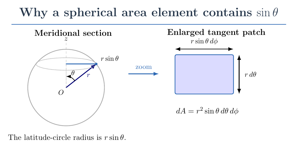
Figure 4. The meridional section shows why a fixed polar angle 𝜃 defines a latitude circle of radius
r sin𝜃. The enlarged local tangent patch then has side lengths rd𝜃 and r sin𝜃dϕ.
The physical spherical displacement is
Hence, on a spherical surface r = constant,
| dar | = r2 sin 𝜃 d𝜃 dϕr, | (38)
|
| dτ | = r2 sin 𝜃 dr d𝜃 dϕ. | (39) |
The sin 𝜃 factor is geometrical: parallels shrink near the poles. It is not a force law and it does not
imply an actual physical source at a pole.
7 Deriving the gradient from the total differential
For a scalar field f(q1,q2,q3), elementary multivariable calculus gives
The gradient is defined geometrically by
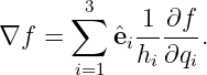
Expand the gradient in the local orthonormal basis:
Insert Equation (10) into Equation (41) and use orthogonality:
Comparing independent coordinate increments with Equation (40),
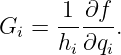
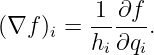
Thus
The scale factor divides a change per coordinate increment by the physical distance associated with
that increment.
8 Divergence: flux through a shrinking coordinate cell
Take a smooth vector field
Consider the pair of faces perpendicular to e1. The positive face is at q1 + dq1 and carries outward
flux approximately
The negative face has the opposite outward normal:
A first-order Taylor expansion yields
There are analogous contributions from the other two pairs of faces.
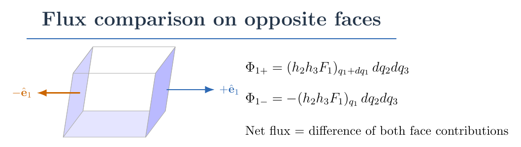
Figure 5. Divergence compares the net outward flux on opposite faces. The face area and the field
component both enter the difference; in curved coordinates the face area generally changes with
position.
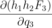
Divide the total outward flux by the physical cell volume h1h2h3dq1dq2dq3 and let the cell
shrink:
∇⋅ F = 1 ____
h1h2h3 | 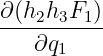 + 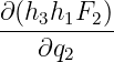 | (50)
|
| +  ![]](https://images.physicslibrary.org/cache/objects/1588/make4ht/CurvilinearFieldGeometryScaleFactorsAndVectorOperators40x.png) . | (51) |
This proof explains the geometry-dependent factors. They arise because a face at one coordinate
value need not have the same area as the opposite face.
9 Curl: circulation around a shrinking coordinate patch
Curl is circulation per unit area, with the loop orientation tied to the surface normal by the
right-hand rule.
Hold q1 fixed and take a tiny loop with sides along q2 and q3. Its positive normal is e1. The two q2
edges contribute their tangential factors h2F2dq2 with opposite traversal directions; the two q3
edges similarly contribute h3F3dq3.
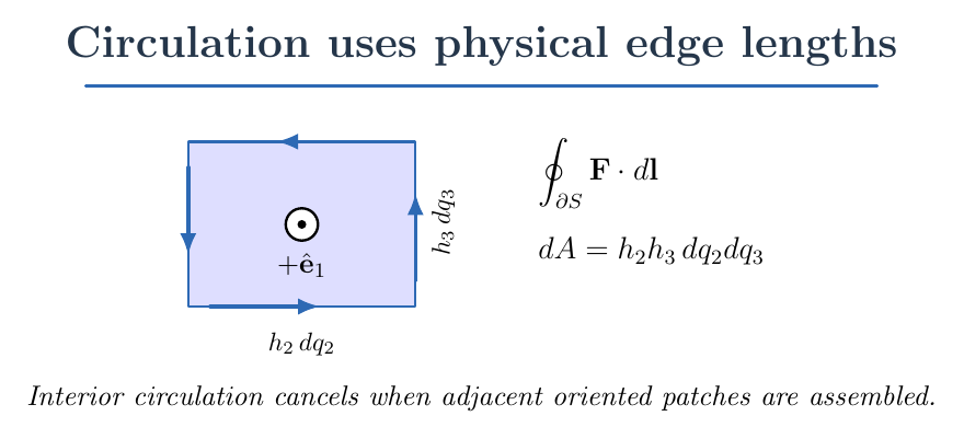
Figure 6. A positively oriented loop in the (q2,q3) coordinate surface measures the first
component of curl. Edge lengths contain scale factors h2 and h3.
Write the circulation around the four sides and group opposing edges. To first order in the patch
area,
| ∮
F ⋅ dl = | 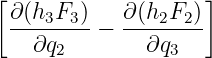 dq2dq3. | (52) |
The physical area is h2h3dq2dq3. Therefore
Cyclically permuting (1, 2, 3) gives
| (∇× F)2 | =  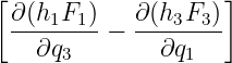 , | (54)
|
| (∇× F)3 | =  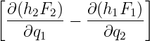 . | (55) |
Notice the contrast: divergence uses physical face areas; curl uses physical edge lengths. Both then
divide by the appropriate physical volume or area.
10 The scalar Laplacian
The scalar Laplacian is defined by
For a gradient field, Equation (45) gives the local components
Insert these into the divergence formula:
∇2f = 1 ____
h1h2h3 |  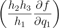 | (58)
|
| + |  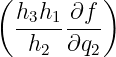 | (59)
|
| + |  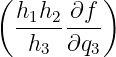 ![]](https://images.physicslibrary.org/cache/objects/1588/make4ht/CurvilinearFieldGeometryScaleFactorsAndVectorOperators56x.png) . | (60) |
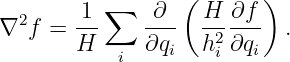
If H = h1h2h3, the same formula is
This conservative form is particularly useful in discretization and finite-volume modeling.
11 Cylindrical vector operators
Set (q1,q2,q3) = (s,ϕ,z) and (h1,h2,h3) = (1,s, 1). The gradient is
The divergence is
∇⋅ F = 1
s + 1
s  +  . | | (63) |
The curl components are
| (∇× F)s | = 1
s −  , | (64)
|
| (∇× F)ϕ | =  −  , | (65)
|
| (∇× F)z | = 1
s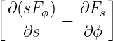 . | (66) |
And the scalar Laplacian becomes
∇2f = 1
s  + 1 _
s2  +  . | | (67) |
Each 1∕s factor reflects the radius-dependent geometry of azimuthal motion and face
areas.
12 Spherical vector operators
Set (q1,q2,q3) = (r,𝜃,ϕ) with
The gradient becomes
| ∇f = | r + 𝜃1
r  | (69)
|
| + ϕ 1 ___
r sin 𝜃 . | (70) |
The divergence is
| ∇⋅ F = | 1_
r2 + 1 ___
r sin 𝜃 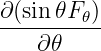 | (71)
|
| + 1 ___
r sin 𝜃 . | (72) |
The curl components are
(∇× F)r = 1 ___
r sin 𝜃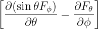 , | | (73)
|
(∇× F)𝜃 = 1
r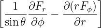 , | | (74)
|
(∇× F)ϕ = 1
r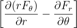 . | | (75) |
Finally,
| ∇2f = | 1_
r2  | (76)
|
| + 1 ____
r2 sin 𝜃 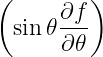 | (77)
|
| + 1 ____
r2 sin 2𝜃 . | (78) |
The r2 in the radial divergence comes from the area of spheres, whereas the sin 𝜃 terms come from
the shrinking latitude circles.
13 Why the basis vectors have derivatives
For cylindrical coordinates,
| s | = cos ϕx + sin ϕy, | (79)
|
| ϕ | = − sin ϕx + cos ϕy. | (80) |
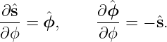
Differentiate term by term:
A vector field F0s therefore changes with angle even if the scalar coefficient F0 is constant.
The analogous spherical relations include
 | = 𝜃, | (82)
|
 | = −r, | (83)
|
 | = sin 𝜃ϕ, | (84)
|
 | = cos 𝜃ϕ, | (85)
|
 | = − sin 𝜃r − cos 𝜃𝜃. | (86) |
These derivatives are not additional physical forces. They record how the chosen basis rotates from
point to point.
14 Worked example 1: a cylindrical scalar field
Let
(The coordinates can be regarded as nondimensional in this mathematical example.)
Differentiate:
 | = 2s cos ϕ, | (88)
|
 | = −s2 sin ϕ, | (89)
|
 | = 4z. | (90) |
Insert the derivatives into Equation (62):
The second term contains one power of s, not two, because an azimuthal derivative must be
divided by hϕ = s. This is the physical distance correction.
15 Worked example 2: divergence of a radial cylindrical field
Let
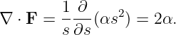
where α is constant. Only Fs = αs is nonzero. Equation (63) gives
Check against the divergence theorem for a cylinder of radius a and length L. On the curved side F
is outward with magnitude αa. Its side area is 2πaL, so
The end caps contribute zero, because F has no z component. The integral of the divergence over
the volume is
The two calculations agree exactly.
16 Worked example 3: the curl of rigid planar rotation
Consider the planar velocity field
where Ω is a constant angular speed. Since vs = vz = 0 and vϕ = Ωs, the only nonzero curl
component is
| (∇× v)z | = 1
s | (97)
|
| = 1
s = 2Ω. | (98) |
A circular contour of radius a supplies an independent Stokes-theorem check:
The area integral of 2Ωz over the disk is also 2πΩa2. This is a classic example of a factor of two
arising from geometry.
17 Worked example 4: the field around a long current
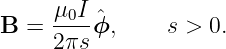
Outside a thin straight wire carrying steady current I along +z, the ideal magnetic field
is
Use the cylindrical curl formula in the region s > 0:
Nevertheless, a circle enclosing the axis has circulation
| ∮
B ⋅ dl | = ∫
02πμ0I
2πs(sdϕ) = μ0I. | (102) |
This is not a contradiction: the axis is excluded from the smooth-field calculation. In the ideal
line-current description the source is distributional,
and the curl has a corresponding distribution concentrated on the axis:
ED05 supplies the language of delta functions needed for that statement; ED04 supplies the
integral-law viewpoint.
18 Worked example 5: spherical radial fields
Take
where β is constant. The spherical divergence formula yields
| ∇⋅ F | = 1 _
r2 (r2βr) | (106)
|
| = 1 _
r2 = 3β. | (107) |
The outward flux through a sphere of radius R is
Integrating the divergence over the ball gives
Again the local and integral calculations agree.
19 Worked example 6: a constant vector in spherical components
A fixed Cartesian vector z can be expressed in spherical components as
Although the coefficients vary with 𝜃, the vector itself is spatially constant. Its divergence must be
zero.
Check directly using Fr = cos 𝜃, F𝜃 = − sin 𝜃, and Fϕ = 0:
| ∇⋅z | = 1 _
r2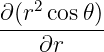 + 1 ___
r sin 𝜃 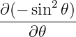 | (111)
|
| = 2 cos 𝜃
r − 2 cos 𝜃
r = 0. | (112) |
The two terms cancel. This is a powerful check that the spherical divergence formula correctly
accounts for the moving basis and the coordinate geometry.
20 Coordinate singularities versus physical singularities
At s = 0, cylindrical azimuth ϕ is undefined. At r = 0 the spherical radial direction is
undefined, and at 𝜃 = 0,π the azimuthal direction is undefined. These are coordinate
singularities.
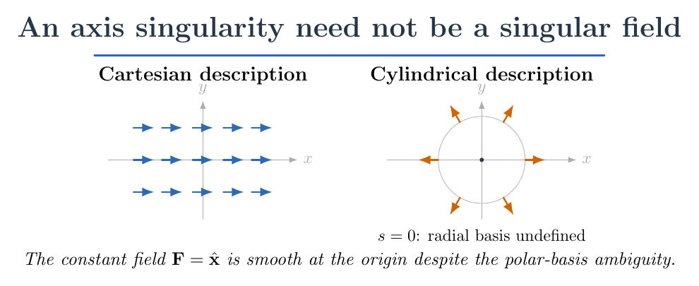
Figure 7. A field can be smooth in Cartesian components even when a cylindrical or spherical
basis becomes undefined at a coordinate axis. A physical singularity requires separate evidence.
For example, F = x is a finite, smooth vector everywhere in Cartesian coordinates. In cylindrical
coordinates,
Both cylindrical basis vectors become ambiguous at s = 0, but the physical field does
not.
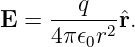
Now compare an ideal point-charge Electric Field,
For r > 0 the spherical divergence formula gives ∇⋅ E = 0. However, the outward flux of any
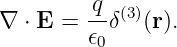
sphere enclosing the origin is q∕𝜖0. The field genuinely becomes unbounded as r → 0, and its source
is a three-dimensional delta function:
The regular-point differential formula alone cannot capture the contribution at the singular source.
This distinction is essential whenever one transforms Maxwell’s equations into curvilinear
coordinates.
21 What coordinate methods do not change
Changing coordinates does not alter a physical flux, circulation, field energy, or force. The
numerical components and integration measures may change, but the resulting invariant scalar
quantity must agree.
As one example, the spherical volume integral of a constant density ρ0 over a ball of radius R
is
| Q | = ∫
V ρ0 dτ | (116)
|
| = ρ0 ∫
0Rr2dr ∫
0π sin 𝜃 d𝜃 ∫
02πdϕ | (117)
|
| = ρ0 (2)(2π) | (118)
|
| = 4πR3
3 ρ0. | (119) |
The answer is simply density times physical volume, whatever coordinates were used to evaluate
it.
22 Connection to numerical field models and EDL measurements
This geometric viewpoint matters outside analytic textbook problems. In a finite-volume
field solver, the flux through a cell face is evaluated using the face’s physical area; a
divergence estimate divides the signed net flux by the cell’s physical volume. In curvilinear
coordinates, omitting a factor such as s or r2 sin 𝜃 changes the numerical conservation
law.
For a laboratory field map, a Hall probe may measure the component B ⋅u along its sensitive axis
u. If the sensor is moved around a wire, a reading interpreted as Bϕ requires knowing the local ϕ
direction. Likewise, an electric potential measured on a circular grid must be differentiated with
respect to physical distance, not an angle alone.
These observations connect the mathematics of ED06 to later magnetic-field mapping, electrostatic
potential reconstruction, and electromagnetic finite-volume calculations.
23 Practice problems
- Reconstruct the cylindrical volume element by calculating the Jacobian
∂(x,y,z)∕∂(s,ϕ,z).
- Starting from r(r,𝜃,ϕ), obtain h𝜃 and hϕ without using a memorized arc-length
formula.
- Use Equation (45) to find the gradient of f = s cos ϕ + z2.
- Evaluate ∇⋅ (s2s) for s > 0 and check with flux through a cylinder.
- Calculate the curl of Fϕ = γs2 with all other cylindrical components zero.
- Apply the spherical Laplacian to f = r2 and verify that ∇2f = 6.
- Show ∇2(1∕r) = 0 for r > 0. Explain why the source at the origin is not ruled out.
- Use spherical divergence to show that r−2r is divergence free away from the origin.
- Express x in cylindrical components and verify its divergence vanishes for s > 0.
- A circular Hall-probe path has radius s. Explain which component the probe must
sense to map an azimuthal magnetic field.
24 Summary and next step
The key starting point is not a table of differential operators. It is the position map r(q1,q2,q3)
and its scale factors
These factors determine the physical line, surface, and volume elements. The gradient follows from
the total differential, divergence from flux through opposite faces, and curl from circulation around
a small loop. Their more complicated cylindrical and spherical forms are therefore geometric
consequences rather than arbitrary algebraic corrections.
ED07 will use divergence, curl, boundary conditions, and decay assumptions to investigate the
Helmholtz question: under what conditions do the divergence and curl of a vector field determine
that field?
References
References
[1] D. J. Griffiths, Introduction to Electrodynamics, 5th ed., Cambridge University Press,
2023.
[2] H. M. Schey, Div, Grad, Curl, and All That, 4th ed., W. W. Norton, 2005.
[3] G. B. Arfken, H. J. Weber, and F. E. Harris, Mathematical Methods for Physicists,
7th ed., Academic Press, 2013.
[4] M. L. Boas, Mathematical Methods in the Physical Sciences, 3rd ed., Wiley, 2006.