Electromagnetic Waves, Antennas, and RF: Boundary Waves - Reflection, Transmission, and
Refraction
EM20 showed how a uniform electromagnetic wave propagates inside a homogeneous material.
Real propagation paths are rarely uniform forever. A wave eventually meets a boundary: air to
glass, air to soil, free space to a radome, dielectric to Conductor, or one layer of a circuit or
antenna structure to another.
At that boundary, Maxwell’s Equations do not permit the fields to change arbitrarily.
Their allowed discontinuities are fixed by the electromagnetic boundary conditions.
Those conditions, together with the plane-wave relation between electric and magnetic
fields, determine how much of the incident wave is reflected, how much is transmitted,
whether the transmitted wave changes direction, and whether a phase reversal occurs
[1, 3, 4, 5].
The central chain developed in this article is
- Maxwell equations;
- boundary conditionse;
- Γ,τ;
- R,T;
- Snell and Fresnel laws;
1 The interface geometry
Let medium 1 occupy z < 0 and medium 2 occupy z > 0. The interface is the plane z = 0, with
unit Normal
pointing from medium 1 into medium 2.
Each medium has constitutive parameters
and therefore its own propagation constant and intrinsic impedance,
For the first derivation we use lossless media, so η1 and η2 are real. The complex-impedance
extension is introduced later.
2 Boundary conditions come directly from Maxwell’s equations
The wave-interface formulas are not separate laws added to Electromagnetism. They follow from
the integral forms of Maxwell’s equations by shrinking the integration surface or contour around
the interface [1, 2, 3].
2.1 Tangential electric field
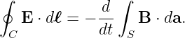
Faraday’s law in integral form is
Take a narrow rectangular contour that straddles the interface. As its height tends to zero, the
enclosed area tends to zero, so the magnetic-flux term vanishes for finite fields. The two long sides
remain, giving
Thus the tangential electric field is continuous across an ordinary interface.
2.2 Tangential magnetic field
Ampere-Maxwell law gives
If a free surface-current density Ks exists at the interface, the limiting contour gives
For the dielectric interfaces considered first,
so the tangential magnetic field is also continuous.
2.3 Normal electric flux density
Gauss’s Law applied to a thin pillbox gives
where ρs is free surface-charge density.
2.4 Normal magnetic flux density
Gauss’s law for magnetism similarly gives
The normal component of B is therefore continuous because magnetic monopole surface charge
does not appear in classical electromagnetism.
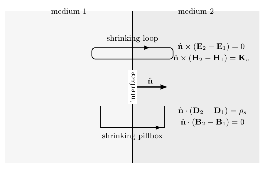
Figure 1. Maxwell boundary conditions at an interface. A narrow loop isolates
tangential-field conditions while a pillbox isolates normal-flux conditions.
3 Normal incidence: incident, reflected, and transmitted waves
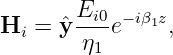
Consider a linearly polarized plane wave incident normally from medium 1. Choose
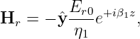
for the incident phasor. The reflected wave propagates in the −z direction,
and the transmitted wave propagates in the +z direction,
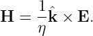
For a uniform plane wave,
Therefore
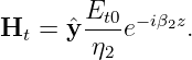
and
The minus sign in Hr is essential: the reflected wave carries energy toward −z.
4 Deriving the normal-incidence reflection coefficient
At z = 0, tangential E is continuous:
Tangential H is also continuous when Ks = 0:
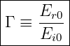
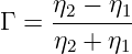
Define the electric-field reflection coefficient
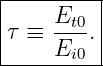
and transmission coefficient
The first boundary condition gives
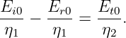
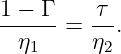
The magnetic-field condition gives
Substitute τ = 1 + Γ:
Collect the Γ terms:
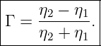
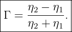
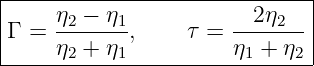
Hence
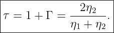
Then
These two compact expressions are the normal-incidence Fresnel amplitude coefficients written in
impedance form.
5 What the sign of the reflection coefficient means
If
then
The reflected electric field is then reversed in sign relative to the incident electric field at the
boundary. For a sinusoid, this is a 180∘ phase reversal.
If
then
and there is no such sign reversal.
If
then
The interface is impedance matched and no plane-wave reflection occurs at normal
incidence.
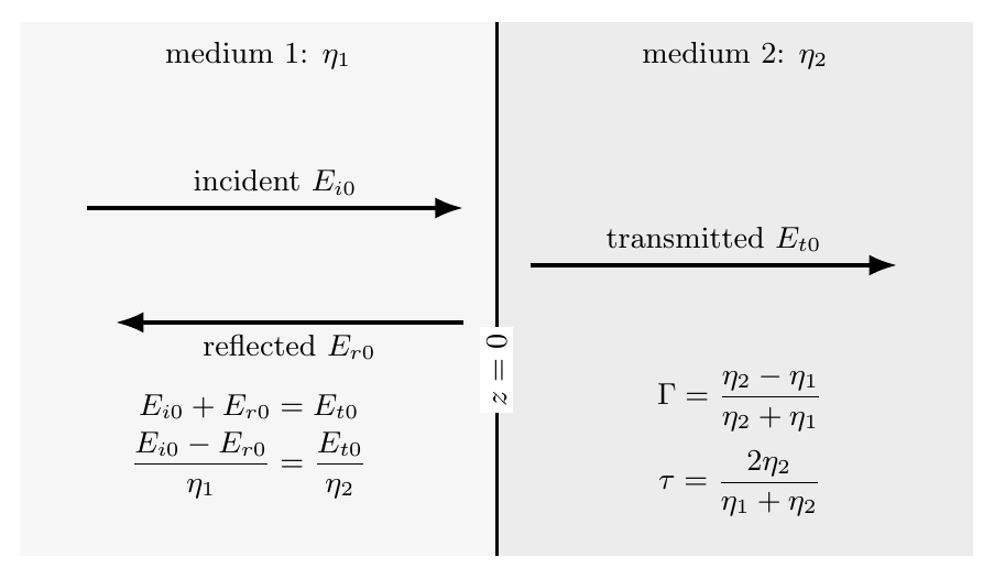
Figure 2. At normal incidence the reflected and transmitted amplitudes are fixed by
continuity of tangential E and H. Reflection occurs when the intrinsic impedances differ.
6 Power reflection and transmission coefficients
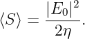
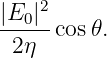
The time-averaged power density of a sinusoidal plane wave in a lossless medium is
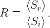
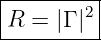
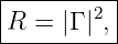
Define the reflected power fraction
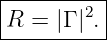
Because the incident and reflected waves are in the same medium,
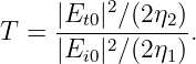
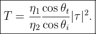
For the transmitted power fraction,
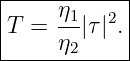
so
Therefore
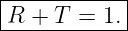
For two lossless media with no absorption at the boundary,
This is simply energy conservation applied to the interface.
7 Example: air into a dielectric with relative permittivity 4
Let medium 1 be air, approximated as free space,
and let medium 2 be a nonmagnetic lossless dielectric with
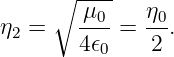
Its intrinsic impedance is
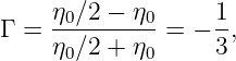
Thus
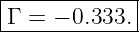
so
The reflected electric field has one-third the incident amplitude and is phase reversed.
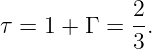
The transmitted electric-field coefficient is
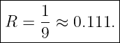
The reflected power fraction is
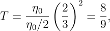
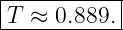
The transmitted power fraction is
so
Notice the important distinction: τ = 2∕3 is a field-amplitude ratio, not a power ratio.
8 Reflection from a lossy medium
The same normal-incidence amplitude formula remains valid when medium 2 has complex intrinsic
impedance:
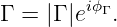
Now Γ is generally complex. Its magnitude gives the reflected field-amplitude fraction and its
argument gives the reflection phase shift:
The transmitted wave also attenuates after entering medium 2 because
Thus two physically distinct effects must be separated:
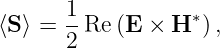
For a general lossy medium at normal incidence, the time-average power flux should be computed
from
rather than by blindly using the lossless expression |E|2∕(2η) with a complex η.
9 Why refraction occurs at oblique incidence
Now let the incident wave strike the boundary at angle 𝜃i measured from the normal. The reflected
and transmitted waves make angles 𝜃r and 𝜃t.
At every point along the interface, the boundary conditions must hold for all time. Therefore the
incident, reflected, and transmitted waves must have the same phase variation parallel to the
interface. If the interface lies along x, phase matching requires
The first equality gives
The second gives
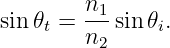
For lossless isotropic media,
so
This is Snell’s law, obtained directly from electromagnetic phase continuity along the
boundary.
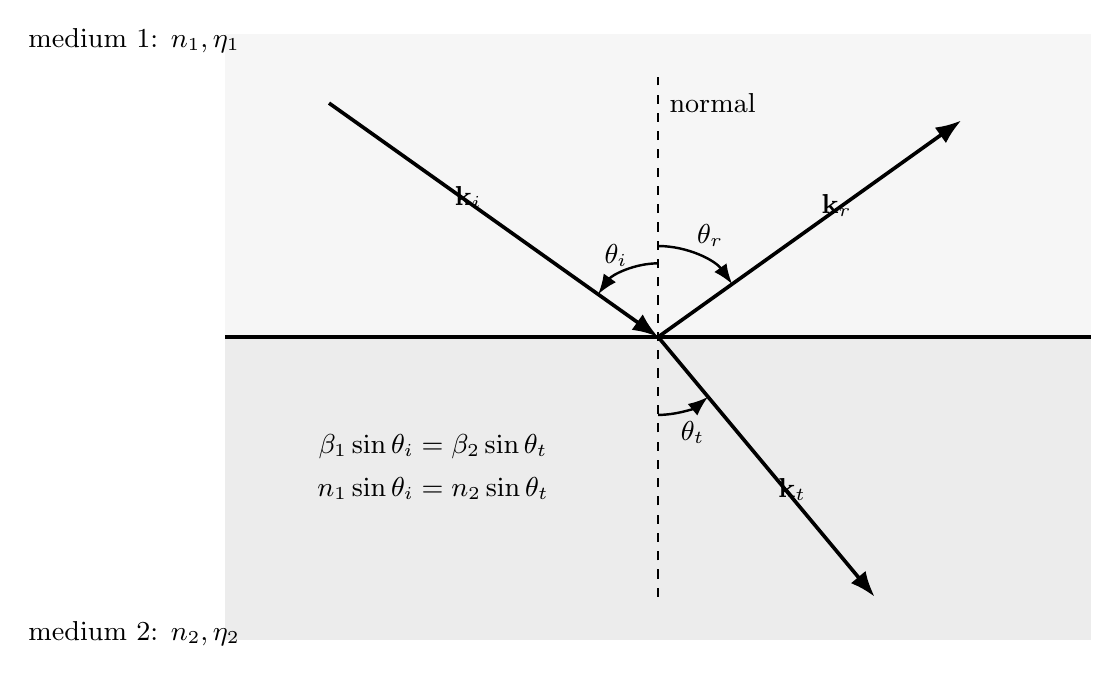
Figure 3. Oblique incidence requires equal tangential phase variation along the interface.
This gives 𝜃r = 𝜃i and Snell’s law.
10 TE and TM polarizations at an interface
At oblique incidence, polarization matters because the electric and magnetic fields project
differently onto the interface.
10.1 TE polarization
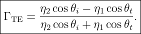
For transverse-electric (TE, or s) polarization, the electric field is perpendicular to the plane of
incidence. Applying the tangential E and H boundary conditions gives
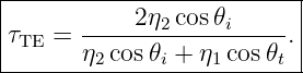
The corresponding electric-field transmission coefficient is
10.2 TM polarization
For transverse-magnetic (TM, or p) polarization, the magnetic field is perpendicular to the plane of
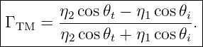
incidence. The electric-field reflection coefficient is
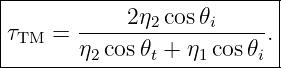
The electric-field transmission coefficient is
At normal incidence,
and both TE and TM reflection coefficients reduce to
11 Power coefficients at oblique incidence
For lossless media, the normal component of average power flow is proportional to
Therefore, for either TE or TM polarization,
and
For lossless interfaces,
The cosine factor appears because the relevant conserved quantity is power crossing the interface,
not power along the slanted propagation direction.
12 Brewster angle
A special feature appears for TM polarization. At one incidence angle the numerator of ΓTM can
vanish:
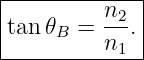
For nonmagnetic lossless media, this occurs at the Brewster angle
At 𝜃i = 𝜃B, an ideal TM-polarized plane wave has zero reflected amplitude.
For air to glass with
This effect is polarization selective: the TE reflection coefficient does not vanish at the same
angle.
13 Critical angle and total internal reflection
Suppose the wave travels from a higher-index medium into a lower-index medium,
Snell’s law requires
At a sufficiently large 𝜃i, the right side would exceed 1 if interpreted as an ordinary propagating
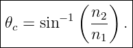
transmitted angle. The limiting incidence angle is the critical angle,
For
there is no propagating transmitted plane wave carrying power away from the boundary in the
usual refracted direction. Instead, the field in medium 2 is evanescent in the normal direction while
the reflection magnitude becomes
The phase of Γ remains nontrivial even though all time-average normal power is reflected. This
phenomenon is total internal reflection.
14 Fresnel reflectance versus angle
For air-to-glass incidence, n1 = 1 and n2 = 1.5. The TE and TM reflection coefficients
behave differently as the incidence angle grows. The TM reflectance falls to zero at the
Brewster angle, while the TE reflectance rises monotonically toward unity near grazing
incidence.
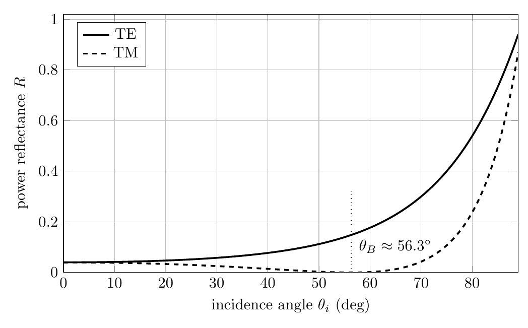
Figure 4. Fresnel power reflectance for an air-to-glass interface. TM reflection vanishes at
the Brewster angle, while both polarizations approach total reflection near grazing incidence.
15 Standing-wave structure on the incident side
When a reflected wave is present, the total electric field in medium 1 is
Using
we obtain
The reflected and incident fields interfere, producing spatial maxima and minima. For a lossless
medium and fixed |Γ| < 1,
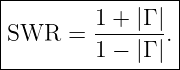
Their ratio is
This same mathematical structure later reappears in transmission-line voltage standing-wave ratio
(VSWR). The transmission-line result is not a coincidence: it is another manifestation of forward
and backward waves meeting an impedance discontinuity.
16 Several important limiting cases
16.1 Matched boundary
If
then at normal incidence
No reflection occurs even though other material properties may differ.
16.2 Perfect electric conductor
For an ideal perfect electric conductor, the tangential electric field at the surface must
vanish. The reflected field therefore cancels the incident tangential electric field at the
boundary:
Hence
This is complete reflection with a 180∘ electric-field phase reversal.
16.3 Very good but finite conductor
A good conductor has a small complex intrinsic impedance compared with free space.
Therefore
but not exactly. A small transmitted field enters the conductor and then decays over the skin
depth developed in EM20.
17 The boundary-wave workflow
A reliable interface calculation can be organized as follows:
- determine 𝜖, μ, and σ in each medium;
- compute γ and η as needed;
- identify the incidence angle and polarization;
- enforce tangential phase matching to obtain reflection and refraction angles;
- apply the appropriate TE or TM Fresnel coefficient;
- convert field-amplitude coefficients into power coefficients with the correct impedance
and angle factors;
- if a transmitted medium is lossy, propagate the transmitted field with e−αz after the
interface.
This workflow keeps three distinct physical mechanisms separate:
- reflection at the boundary;
- refraction at the boundary;
- attenuation inside the material
18 Connection to RF systems and antennas
Boundary-wave physics appears throughout RF engineering. Examples include radomes, dielectric
antenna substrates, soil and seawater propagation, building penetration, microwave windows,
coaxial and waveguide discontinuities, and the transition from an antenna’s near environment into
free space.
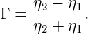
The reflection coefficient also foreshadows impedance matching in circuit and transmission-line
language. At normal incidence,
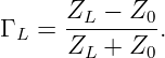
has exactly the same algebraic form as the voltage reflection coefficient at a transmission-line
load,
The common structure arises because both problems enforce continuity relations between paired
wave variables and their impedance ratios.
19 What EM21 adds to the series
EM20 described propagation within one uniform medium. EM21 adds the physics of crossing
between media. The key results are
for normal incidence,
and the TE/TM Fresnel coefficients for oblique incidence.
These results establish the mathematical foundation for multilayer propagation, transmission lines,
Standing Waves, impedance matching, waveguides, radomes, and antenna-to-medium
coupling. The natural companion is an EM21E1 problem set devoted to boundary-condition
derivations, Fresnel coefficients, Brewster angle, total internal reflection, and power
bookkeeping.
References
References
[1] D. J. Griffiths, Introduction to Electrodynamics, 4th ed., Cambridge University Press,
2017.
[2] J. D. Jackson, Classical Electrodynamics, 3rd ed., Wiley, 1999.
[3] D. K. Cheng, Field and Wave Electromagnetics, 2nd ed., Addison-Wesley, 1989.
[4] F. T. Ulaby and U. Ravaioli, Fundamentals of Applied Electromagnetics, 7th ed.,
Pearson, 2015.
[5] C. A. Balanis, Advanced Engineering Electromagnetics, 2nd ed., Wiley, 2012.
[6] D. M. Pozar, Microwave Engineering, 4th ed., Wiley, 2012.