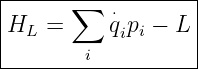
Calculus of Variations: Hamilton's Principle and Classical Mechanics

(Topic)

Calculus of Variations: Hamilton’s Principle and Classical Mechanics

The calculus of variations becomes a mechanics principle when the independent variable is time and the quantity being varied is an entire trajectory. Instead of asking which curve minimizes geometric length or elastic energy, we ask which path through configuration space makes the action stationary.

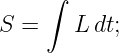
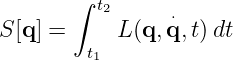
Hamilton’s principle states, in its standard fixed-endpoint form,

|----------------------------------| | ∫ t2 ⋅ | δS = 0, S[q] = L(q, q,t)dt| ---------------------t1--------------

(1)

for all admissible variations that keep the initial and final configurations fixed. Here L is the Lagrangian and q = (q₁,…,q_n) denotes generalized coordinates.

The principle does not say that the physical path always minimizes the action. The physical path is stationary. Depending on the interval and the system, it may be a minimum, a maximum, a saddle, or a degenerate stationary path. CV11–CV13 developed the mathematical tools needed to make that distinction.

Hamilton’s 1834 and 1835 essays placed action and characteristic functions at the center of dynamics [1, 2]. The modern fixed-time stationary-action formulation used here is standard in analytical mechanics texts such as Lanczos, Goldstein, Landau and Lifshitz, and Arnold [4, 5, 6, 7].

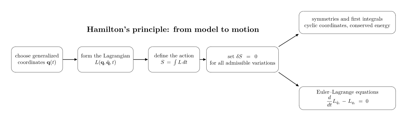
Figure. Hamilton’s principle converts a mechanical model into a variational problem. Once the Lagrangian is known, the stationarity calculation produces the equations of motion and exposes the quantities associated with symmetry.

1 Learning objectives

After completing this entry, the reader should be able to:

define the action functional and state Hamilton’s principle precisely for fixed endpoint times and configurations;
derive the Euler–Lagrange equations of classical mechanics from the first variation of the action;
recover Newton’s second law for a particle moving in a potential;
distinguish stationary action from least action;
interpret generalized momentum as the boundary coefficient ∂L∕∂_i;
derive conservation of a generalized momentum from a cyclic coordinate;
derive the conserved energy function for an autonomous Lagrangian;
formulate and solve the free-particle, uniform-gravity, harmonic-oscillator, pendulum, and central-force examples;
explain how generalized coordinates encode geometry without changing the variational logic;
connect Hamilton’s principle with the second variation, conjugate points, Noether-type ideas, and the later Hamiltonian formulation.

2 Historical bridge from variational geometry to mechanics

Variational reasoning entered mechanics long before Hamilton. Euler’s 1744 Methodus inveniendi lineas curvas systematized problems in which an integral quantity is extremized over curves [3]. Lagrange then developed a general analytical mechanics in which coordinates and virtual displacements replaced much of the geometric force construction.

Hamilton’s contribution was not merely to repeat the Euler–Lagrange calculation. His 1834 and 1835 papers introduced characteristic and principal functions that encoded the dynamics in a single scalar function and anticipated the Hamilton–Jacobi formulation [1, 2]. In modern language, Hamilton’s principle can be presented as

mechanical trajectory =⇒ stationary point of an action functional.

(2)

This is one reason variational mechanics became a bridge to geometrical optics, continuum mechanics, field theory, quantum mechanics, and optimal control.

3 The action functional

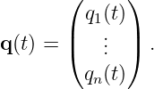
Let a mechanical system be described by generalized coordinates

( ) q (t) | 1. | q (t) = ( .. ) . qn(t)

(3)

A Lagrangian is a scalar function

⋅ L = L (q,q,t).

(4)

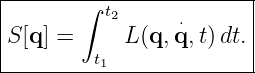
The action of a trajectory between fixed times t₁ and t₂ is

|-------∫--t2-------------| |S [q ] = L (q,q⋅,t) dt.| | t1 | -------------------------|

(5)

The input to S is an entire trajectory. The output is one real number. Thus S is a functional in exactly the sense developed in CV01.

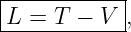
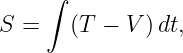
For a standard conservative system,

|-----------| |L = T − V , -------------

(6)

where T is kinetic energy and V is potential energy.

The minus sign is fundamental. Hamilton’s principle does not extremize the total mechanical energy T + V . It makes stationary the time integral of T − V .

4 Admissible variations of a mechanical trajectory

Consider a one-parameter family

q𝜀(t) = q∗(t) + 𝜀η (t),

(7)

where q_∗ is a candidate physical trajectory and η is an admissible variation.

For fixed endpoint configurations,

|------------------------| η (t1) = 0, η(t2) = 0.| --------------------------

(8)

The endpoint times are also fixed in the standard form developed here.

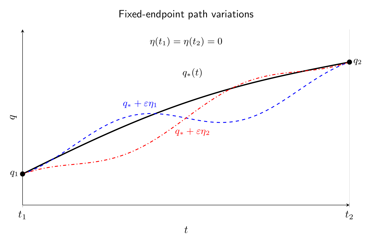
Figure. The physical trajectory is compared with nearby admissible trajectories that pass through the same endpoint configurations at the same endpoint times. The varied paths need not satisfy the equations of motion.

The varied velocity is

⋅q = q⋅ + 𝜀η⋅. 𝜀 ∗

(9)

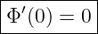
The scalarized action is

Φ (𝜀) = S[q∗ + 𝜀η ].

(10)

Hamilton’s principle requires

|--′-------| -Φ-(0)-=-0-|

(11)

for every admissible η.

5 Deriving the equations of motion

Write

∫ t2 ⋅ ⋅ S[q𝜀] = L(q∗ + 𝜀η, q∗ + 𝜀η,t)dt. t1

(12)

Differentiate with respect to 𝜀 and evaluate at 𝜀 = 0:

∫ t2[∑n ∑n ] δS = Lq ηi + L ⋅⋅ηi dt. t1 i=1 i i=1 qi

(13)

Integrate the velocity-variation term by parts:

∫ t2 ⋅ [ ]t2 ∫ t2 d ( ) L ⋅qiηidt = L ⋅qiηi − -- L⋅qi ηidt. t1 t1 t1 dt

(14)

The fixed-endpoint conditions make the boundary term vanish. Therefore

n ∫ [ ] ∑ t2 d-( ) δS = Lqi − dt L⋅qi ηi dt. i=1 t1

(15)

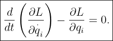
Because the components η_i may be chosen independently, the Fundamental Lemma gives

|---(----)-----------------------------| |d ∂L ∂L | |-- -⋅-- − --- = 0, i = 1,...,n.| |dt ∂qi ∂qi | ---------------------------------------

(16)

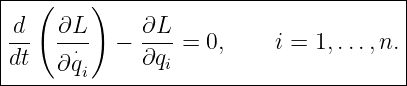
These are the Lagrange equations of motion.

6 Recovering Newton’s second law

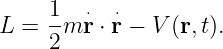
For a particle of mass m with Cartesian position r = (x,y,z) in a potential V (r,t),

L = 1m ⋅r ⋅ ⋅r − V (r,t). 2

(17)

For the x coordinate,

∂L ⋅ ∂L ∂V --⋅ = m x, ∂x- = − -∂x-. ∂ x

(18)

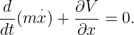
Hence

d ⋅ ∂V --(m x) + ----= 0. dt ∂x

(19)

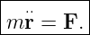
Repeating for all components gives

|------------| |m ⋅⋅r = − ∇V. | --------------

(20)

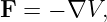
Since the conservative force is

F = − ∇V,

(21)

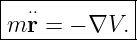
we recover

|--⋅⋅-----| m-r-=--F.-

(22)

Thus Newtonian mechanics and Hamilton’s principle are equivalent for this class of systems, but they organize the calculation differently.

7 Why the principle says stationary action, not least action

The phrase “principle of least action” is common historically, but it is potentially misleading in the present fixed-time formulation. The mathematical condition obtained from the first variation is

δS = 0,

(23)

not

S = minimum.

(24)

CV11 showed that classification requires the second variation. CV12 showed that conjugate points can destroy the minimizing character of an extremal over a sufficiently long interval. CV13 showed that strong minimality also requires finite-slope control.

For the harmonic oscillator, for example, the classical trajectory can cease to be minimizing once the time interval reaches the first conjugate time even though the Euler–Lagrange equation remains perfectly valid.

Thus the careful statement is

|------------------------------------------| -physical path-makes-the-action-stationary.-|

(25)

8 Generalized momentum comes from the boundary term

The integration-by-parts boundary term contains

∂L --⋅ηi. ∂qi

(26)

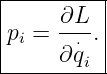
This motivates the definition

|---------| | ∂L | pi = --⋅. | -----∂qi---

(27)

The quantity p_i is the generalized momentum conjugate to q_i.

In Cartesian particle mechanics,

px = m x⋅,

(28)

so generalized momentum reduces to ordinary linear momentum. In curvilinear or constrained coordinates it may take a less obvious form.

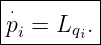
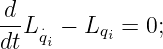
The Lagrange equation can be written

|--------| p⋅ = L .| --i----qi--

(29)

This form immediately reveals the connection between coordinate dependence and momentum change.

9 Cyclic coordinates and conserved momentum

Suppose the Lagrangian does not depend explicitly on one coordinate q_j:

∂L--= 0. ∂qj

(30)

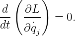
Then the Lagrange equation becomes

( ) -d ∂L⋅- = 0. dt ∂qj

(31)

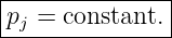
Therefore

|p-=--constant.| --j-------------

(32)

A coordinate absent from the Lagrangian is called cyclic or ignorable. The corresponding generalized momentum is conserved.

This is the mechanics version of the cyclic-coordinate first integral developed in CV06. CV20 will place it inside Noether’s theorem, where continuous symmetries generate conservation laws systematically.

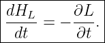
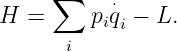
10 Time independence and the energy first integral

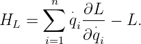
Define

n ∑ ⋅∂L-- HL = qi ⋅ − L. i=1 ∂ qi

(33)

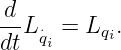
Differentiate along an Euler–Lagrange trajectory:

dHL--= ∑ ⋅⋅q L⋅ + ∑ ⋅q d-L ⋅ − dL-. dt i qi idt qi dt i i

(34)

But

dL ∑ ⋅ ∑ ⋅⋅ --- = Lt + Lqiqi + Lq⋅qi. dt i i i

(35)

The acceleration terms cancel, and the Euler–Lagrange equations give

d --L ⋅qi = Lqi. dt

(36)

Therefore

|--------------| |dHL-- ∂L- | --dt--=--−-∂t-.|

(37)

If the Lagrangian has no explicit time dependence,

|----------------| |HL = constant. | -----------------

(38)

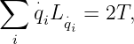
For a natural mechanical system with

L = T − V

(39)

and a kinetic energy quadratic in the velocities,

∑ ⋅q L⋅ = 2T, i qi i

(40)

HL = 2T − (T − V ) = T + V.

(41)

Hence

|-----------------------| E--=-T-+-V--=-constant.--

(42)

This is the mechanical interpretation of the Beltrami/energy first integral introduced in CV06.

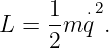
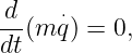
11 Example: the free particle

Consider one-dimensional motion with

1 2 L = -m q⋅. 2

(43)

The Euler–Lagrange equation is

d-(m ⋅q) = 0, dt

(44)

|------| |⋅⋅ | -q =-0.-

(45)

For

q(t1) = q1, q(t2) = q2,

(46)

the stationary path is

|---------------------------| q (t) = q + q2 −-q1(t − t ).| -∗-------1---t2 −-t1-----1---

(47)

The velocity is constant. In configuration space, the free particle follows a straight line.

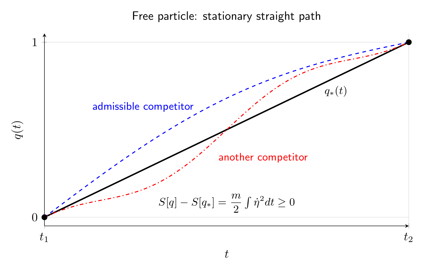
Figure. For fixed spacetime endpoints, the free-particle trajectory is linear in time. A smooth admissible perturbation changes the path while leaving the two endpoints fixed.

This example is stronger than mere stationarity. Write

q = q∗ + η, η(t1) = η (t2) = 0.

(48)

Then

∫ m- t2( ⋅ ⋅ ⋅2) S[q] − S [q∗] = 2 2q∗η + η dt. t1

(49)

Since ⋅
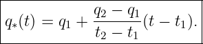
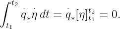
q _∗ is constant,

∫ t2 ⋅q∗⋅η dt = ⋅q∗[η]tt21 = 0. t1

(50)

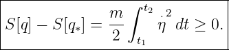
Therefore

|----------------∫--t2----------| S [q] − S [q ] = m ⋅η2dt ≥ 0.| | ∗ 2 t1 | --------------------------------

(51)

Thus the straight free-particle path is the unique global minimizer of the kinetic action for fixed endpoints and fixed endpoint times.

12 Example: uniform gravity

Let y measure upward vertical position. With gravitational potential

V = mgy,

(52)

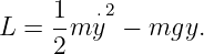
the Lagrangian is

1 ⋅2 L = --m y − mgy. 2

(53)

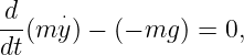
The Euler–Lagrange equation gives

-d(m ⋅y) − (− mg ) = 0, dt

(54)

|⋅⋅-------| -y-=-−-g.-

(55)

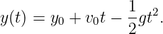
Integrating twice,

y(t) = y0 + v0t − 1gt2. 2

(56)

The usual parabolic kinematics therefore follow directly from stationary action.

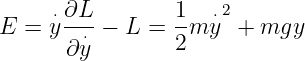
Because L has no explicit time dependence,

⋅∂L 1 ⋅2 E = y--⋅ − L = -m y + mgy ∂ y 2

(57)

is constant.

13 Example: the harmonic oscillator

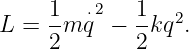
For a mass-spring system,

1- ⋅2 1- 2 L = 2 m q − 2kq .

(58)

The Euler–Lagrange equation is

⋅⋅ m q + kq = 0.

(59)

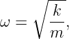
Defining

∘ --- ω = k-, m

(60)

the general solution is

|--------------------------| -q(t) =-A-cosωt-+-B-sinωt.-|

(61)

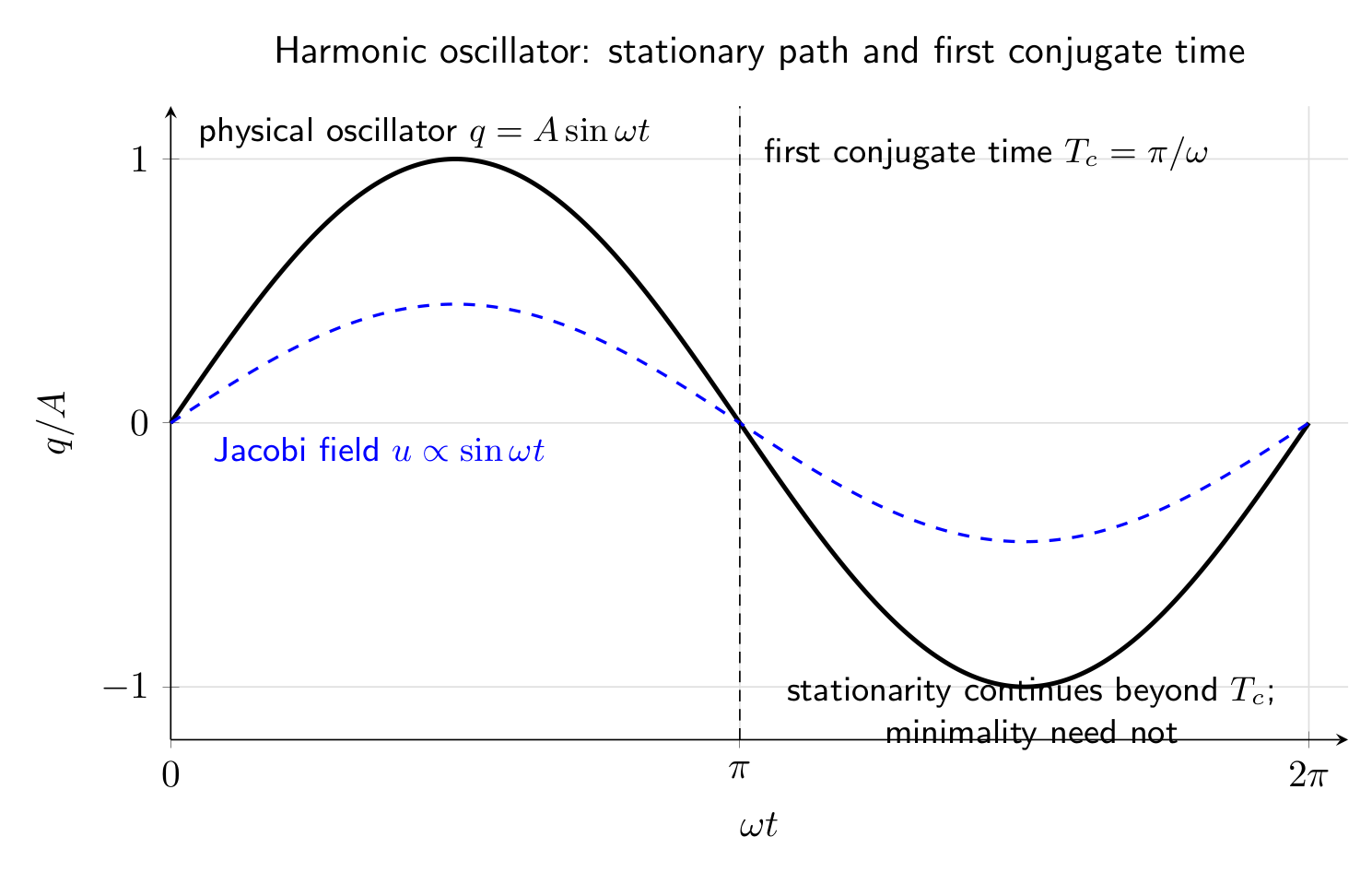
Figure. The oscillator trajectory makes the action stationary. The first conjugate time π∕ω marks the interval length at which the second variation first develops a nontrivial zero direction, so stationary does not mean minimizing for all time intervals.

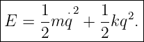
The conserved energy is

|------------------| | 1- ⋅2 1- 2 | E = 2 m q + 2kq .| --------------------

(62)

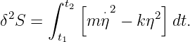
The second variation is

∫ t2[ 2 ] δ2S = m η⋅ − kη2 dt. t1

(63)

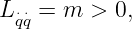
The derivative coefficient is positive,

L ⋅qq⋅= m > 0,

(64)

but this alone does not guarantee a minimum. CV12 showed that the first conjugate time is

|--------| |Tc = π-.| ------ω--|

(65)

This example is one of the clearest demonstrations of why mechanics requires the language of stationary action rather than naive least action.

14 Example: the simple pendulum

Let 𝜃 be the angular displacement of a mass m on a massless rod of length ℓ.

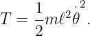
The speed is

⋅ v = ℓ𝜃,

(66)

1- 2 ⋅2 T = 2m ℓ 𝜃 .

(67)

Choosing the lowest point as zero potential,

V = mg ℓ(1 − cos 𝜃).

(68)

Thus

1- 2⋅2 L = 2m ℓ 𝜃 − mg ℓ(1 − cos 𝜃).

(69)

Now

2⋅ L ⋅𝜃 = m ℓ 𝜃, L 𝜃 = − mg ℓsin 𝜃.

(70)

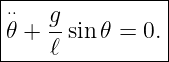
The Euler–Lagrange equation gives

2⋅⋅ m ℓ 𝜃 + mg ℓsin𝜃 = 0,

(71)

hence

|---------------| ⋅𝜃⋅+ g-sin𝜃 = 0. | ----ℓ------------

(72)

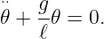
For small angles,

sin𝜃 ≈ 𝜃,

(73)

and the pendulum reduces to a harmonic oscillator:

⋅⋅ g 𝜃 + -𝜃 = 0. ℓ

(74)

The example illustrates one advantage of generalized coordinates: the single angle 𝜃 automatically incorporates the fixed-length geometric constraint.

15 Generalized coordinates are not Cartesian coordinates in disguise

The derivation of the Euler–Lagrange equations never required the q_i to be Cartesian coordinates. They may be angles, lengths, modal amplitudes, or any smooth coordinates that parameterize the configuration space.

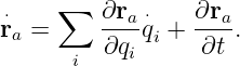
For a system with position vectors

ra = ra(q, t),

(75)

the velocities follow from the chain rule:

⋅ ∑ ∂ra-⋅ ∂ra- ra = ∂qiqi + ∂t . i

(76)

Substitution into the kinetic energy produces a Lagrangian written directly in generalized coordinates.

This is one of the major practical advantages of analytical mechanics: geometry enters through the coordinate map and the kinetic energy rather than through separate Cartesian constraint forces. CV15 will develop this systematically.

16 Example: central-force motion and angular momentum

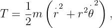
Consider a particle moving in a plane under a central potential V (r). In polar coordinates,

( ) 1- ⋅2 2⋅2 T = 2m r + r 𝜃 ,

(77)

( ) 1- ⋅2 2⋅2 L = 2m r + r 𝜃 − V(r).

(78)

The angle 𝜃 does not appear explicitly:

L 𝜃 = 0.

(79)

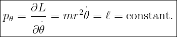
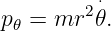
Therefore

|--------------------------------| | ∂L- 2⋅ | p 𝜃 = ⋅= mr 𝜃 = ℓ = constant.| ------∂𝜃--------------------------

(80)

This is the conserved angular momentum about the force center.

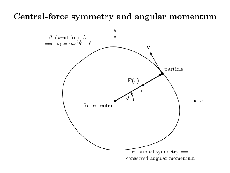
Figure. For a central potential, rotation of the coordinate angle leaves the Lagrangian unchanged. The cyclic coordinate 𝜃 therefore produces conserved angular momentum p_𝜃 = mr² ⋅
𝜃 .

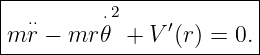
The radial Euler–Lagrange equation is

( ) -d ⋅ ⋅2 ′ dt(m r) − mr 𝜃 − V (r) = 0,

(81)

|---------⋅2-------------| |m ⋅⋅r − mr 𝜃 + V ′(r) = 0.| -------------------------|

(82)

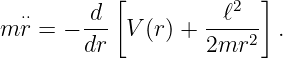
Using the conserved angular momentum,

⋅ --ℓ- 𝜃 = mr2 ,

(83)

so the radial dynamics can be written

⋅⋅ d [ ℓ2 ] m r = − --- V (r) + ----2- . dr 2mr

(84)

The term

2 --ℓ--- 2mr2

(85)

acts as a centrifugal contribution to the effective potential.

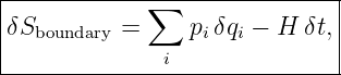
17 The boundary differential and a preview of Hamiltonian mechanics

When endpoint positions are allowed to vary while the endpoint times remain fixed, the first variation contains the boundary term

∑ piδqi. i

(86)

If endpoint time also varies, the more complete endpoint differential becomes

|------------∑---------------| δS = p δq − H δt,| | boundary i i | --------------i---------------

(87)

where

∑ ⋅ H = piqi − L. i

(88)

This relation is a preview rather than a full derivation. Its importance is that the action itself begins to behave like a generating function whose derivatives produce momenta and energy. Hamilton’s 1835 “principal function” develops this idea historically [2]. CV22 will return to it when passing from Lagrangian to Hamiltonian mechanics.

18 Symmetry is already visible before Noether’s theorem

Two conservation laws have now emerged almost automatically:

if q_j does not appear explicitly in L, then p_j is conserved;
if t does not appear explicitly in L, then H_L is conserved.

These statements are early forms of a broader principle:

|------------------------------------------------| -continuous-symmetry-----⇐⇒-----conservation--law.-|

(89)

CV20 will formulate this precisely as Noether’s theorem. For now, Hamilton’s principle provides the natural setting in which the pattern becomes visible.

19 Why variational mechanics is useful

Newton’s laws are often the fastest tool for a simple Cartesian particle. Hamilton’s principle becomes increasingly valuable when the system has geometry, many degrees of freedom, or hidden symmetries.

Some advantages are:

coordinate flexibility: generalized coordinates may be chosen to fit the geometry;
constraint reduction: holonomic constraints can often be built directly into the coordinates;
scalar formulation: one scalar Lagrangian generates an entire system of differential equations;
symmetry visibility: cyclic coordinates expose conserved quantities immediately;
extension to fields: the same variational logic generalizes to continuum and field theories;
bridge to Hamiltonian mechanics: generalized momenta arise naturally from the boundary terms;
bridge to modern physics: action principles remain central in relativity, quantum theory, and gauge fields.

20 Common misconceptions

20.1 Misconception 1: the physical path always has the smallest action

False. Hamilton’s principle gives stationarity. Classification requires second-variation and related tests.

20.2 Misconception 2: the action is the total energy integrated over time

False. For a standard conservative system,

∫ S = (T − V )dt,

(90)

not ∫ (T + V )dt.

20.3 Misconception 3: the varied paths are possible motions

Not necessarily. The comparison curves need only satisfy the admissibility and endpoint conditions. They generally do not satisfy the equations of motion.

20.4 Misconception 4: generalized momentum always equals m

Only in special coordinates. In general,

pi = L ⋅. qi

(91)

For example, in central-force polar coordinates,

2 ⋅ p𝜃 = mr 𝜃.

(92)

20.5 Misconception 5: energy conservation is imposed separately

For an autonomous Lagrangian, it follows directly from the Euler–Lagrange equations and time-translation invariance.

21 A practical workflow for mechanical variational problems

For a finite-dimensional mechanical system:

choose generalized coordinates q₁,…,q_n;
compute the kinetic energy T;
compute the potential energy V ;
form
$L = T − V ;$ (93)
define the action
$∫ S = L dt;$ (94)
identify the endpoint conditions;
compute
$d --L ⋅ − Lqi = 0; dt qi$ (95)
inspect L for cyclic coordinates and explicit time dependence;
use the resulting first integrals whenever they reduce the problem;
if the question asks whether the stationary path is actually minimizing, apply the CV11–CV13 classification tools.

22 What CV15 adds

This article has used generalized coordinates but has not yet developed constraints systematically. CV15 will study constraints and generalized coordinates in mechanics in more depth, including coordinate reduction, holonomic constraints, constraint forces, and variational formulations with multipliers.

The progression is therefore

|----------------------------------------------------------------------| CV14: stationary action −→ CV15: constrained mechanical coordinates| | | ------------------−→--CV22:--Hamiltonian--formulation-------------------

(96)

Summary

Hamilton’s principle states that the physical trajectory makes the action

∫ t2 ⋅ S [q] = L(q,q, t)dt t1

(97)

stationary under admissible fixed-endpoint variations.

The first variation yields

|--(----)-------------| |d ∂L ∂L | -- --⋅- − --- = 0. | dt---∂qi-----∂qi-------

(98)

For L = T − V , these equations reproduce Newtonian dynamics while remaining valid in generalized coordinates.

The boundary coefficient

|--------| -pi =-L⋅qi-

(99)

is the generalized momentum. If q_i is cyclic, p_i is conserved. If L is autonomous, then

|------∑---⋅-------| |HL = qipi − L | --------i----------|

(100)

is conserved and equals T + V for standard natural systems.

The free particle, uniform gravity, harmonic oscillator, pendulum, and central-force examples all follow from the same variational template. Most importantly, Hamilton’s principle requires stationary action; whether that stationary trajectory is a minimum is a separate question answered by the second-variation, Jacobi, Weierstrass, and sufficiency theory developed in CV11–CV13.

References

[1] William Rowan Hamilton, “On a General Method in Dynamics; by which the Study of the Motions of all Free Systems of Attracting or Repelling Points is Reduced to the Search and Differentiation of One Central Relation, or Characteristic Function,” Philosophical Transactions of the Royal Society of London, Part II (1834), pp. 247–308.

[2] William Rowan Hamilton, “Second Essay on a General Method in Dynamics,” Philosophical Transactions of the Royal Society of London, Part I (1835), pp. 95–144.

[3] Leonhard Euler, Methodus inveniendi lineas curvas maximi minimive proprietate gaudentes, Lausanne and Geneva: Marcum-Michaelem Bousquet, 1744.

[4] Cornelius Lanczos, The Variational Principles of Mechanics, 4th ed., Dover Publications, 1986.

[5] Herbert Goldstein, Charles Poole, and John Safko, Classical Mechanics, 3rd ed., Addison-Wesley, 2002.

[6] L. D. Landau and E. M. Lifshitz, Mechanics, 3rd ed., Butterworth-Heinemann, 1976.

[7] V. I. Arnold, Mathematical Methods of Classical Mechanics, 2nd ed., Springer, 1989.

[8] I. M. Gelfand and S. V. Fomin, Calculus of Variations, Dover Publications, 2000.

"Calculus of Variations: Hamilton's Principle and Classical Mechanics" is owned by bloftin.
(view preamble)

Calculus of Variations: Hamilton's Principle and Classical Mechanics