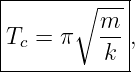
Calculus of Variations: The Jacobi Equation and Conjugate Points
CV11 introduced the second variation and showed that the Legendre condition
is necessary for a weak local minimum. It also exposed a serious limitation: a positive coefficient of
(η′)2 does not guarantee that the whole quadratic form is positive. The sign of the second variation
can depend on the length of the interval.
CV12 develops the classical remedy. The quadratic functional associated with the second variation
has its own Euler–Lagrange equation. That differential equation is the Jacobi accessory equation.
Its zeros reveal conjugate points, locations at which the second variation loses strict
positivity.
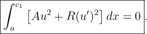
The resulting logic is
Jacobi’s 1837 work supplied the missing interval test that earlier Euler–Lagrange and Legendre
conditions did not provide [7, 5, 6]. Modern treatments include [1, 2, 3, 4].
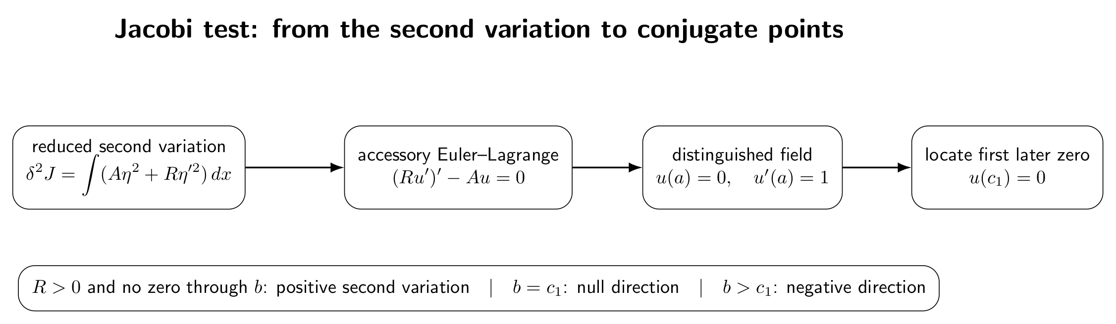
Figure. The Jacobi test begins with the reduced second variation, derives an auxiliary
differential equation, and then uses zeros of its distinguished solution to detect the first loss
of positive definiteness.
1 Learning objectives
After completing this entry, the reader should be able to:
- derive the Jacobi equation from the reduced second variation;
- explain why the Jacobi equation is an Euler–Lagrange equation for an accessory
functional;
- define a conjugate point and compute the first conjugate point in simple problems;
- distinguish an interior conjugate point from a conjugate point occurring exactly at the
terminal endpoint;
- use Jacobi’s factorization identity to understand positivity of the second variation;
- interpret Jacobi fields as infinitesimal separations between neighboring extremals;
- connect conjugate points with Sturm–Liouville eigenvalues and the loss of positive
definiteness;
- apply the theory to the harmonic-oscillator action;
- recognize the geometric meaning of conjugate points in the great-circle example.
2 Starting point: the reduced second variation
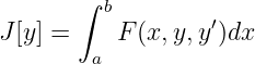
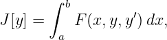
Consider the first-order fixed-endpoint functional
and suppose y∗ is a sufficiently smooth stationary extremal. For a fixed-endpoint variation
CV11 obtained
where all derivatives of F are evaluated along
Integrating the mixed term by parts gives the reduced form
with
The strengthened Legendre condition is
That condition controls the highest-derivative contribution, but it does not determine the sign
of
after integration over an entire interval. If A is negative enough, a sufficiently slowly varying
perturbation can make the integral negative.
3 The accessory functional
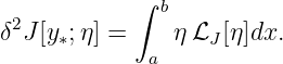
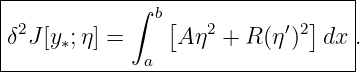
The reduced second variation is itself a functional of the perturbation η. Define
on the class
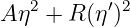
The integrand of this auxiliary problem is
Its partial derivatives are
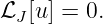
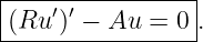
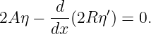
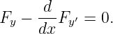
Therefore the Euler–Lagrange equation for the accessory functional is
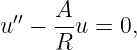
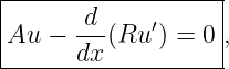
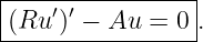
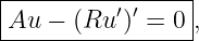
Dividing by 2 and renaming the unknown function u gives
or equivalently,
This is the Jacobi equation or Jacobi accessory equation.
3.1 Why the accessory equation matters
The Jacobi equation is not an unrelated differential equation appended to the original variational
problem. It is the Euler–Lagrange equation of the quadratic functional that determines the
second-order change in J.
Thus there are two Euler–Lagrange equations in the story:
- the original Euler–Lagrange equation determines stationary candidates y∗;
- the Jacobi equation determines critical directions of the second variation around y∗.
This distinction is fundamental.
4 The distinguished Jacobi field
The Jacobi equation is a homogeneous linear second-order ODE. Under the usual regularity
assumptions, there is a unique solution for any two initial data.
To study conjugacy to the left endpoint a, choose the normalized solution
The normalization u′(a) = 1 is only a convenient scale choice. Any nonzero value of u′(a) produces
the same zero locations.
We will call u the distinguished Jacobi field from a.
5 Conjugate points
Definition. A point c > a is conjugate to a along the extremal y∗ if there exists a nontrivial
solution u of the Jacobi equation satisfying
Equivalently, with the normalized distinguished field defined above, the conjugate points are
precisely its zeros after a.
The first conjugate point c1 is the smallest c > a for which
If no such point exists, we say that there is no conjugate point to a on the interval under
consideration.
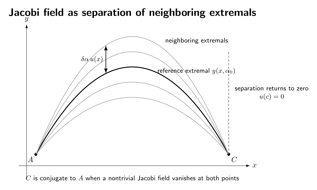
Figure. A Jacobi field can be viewed as the infinitesimal separation between neighboring
extremals. When the separation vanishes again, the neighboring extremals refocus. That
refocusing point is conjugate to the starting point.
6 Jacobi fields from neighboring extremals
The preceding geometric statement can be derived directly. Suppose
is a smooth one-parameter family of extremals of the original functional. For every
α,
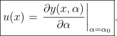
Define the infinitesimal separation field
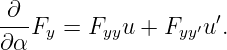
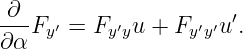
Differentiate the Euler–Lagrange equation with respect to α. The first term gives
The second term gives
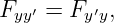
Assuming the mixed derivatives agree,
we obtain
Expand the total derivative of the first product:
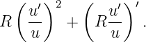
The Fyy′u′ terms cancel, leaving
Using A and R,
which is exactly the Jacobi equation.
Thus the Jacobi equation is also the linearized Euler–Lagrange equation. It describes how an
extremal changes when we move infinitesimally to a neighboring extremal.
7 Jacobi’s factorization identity
The deepest algebraic connection between the Jacobi equation and positivity of the second
variation is a factorization identity.
Suppose u is a nonzero solution of
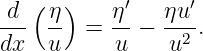
on an interval where u≠0. Then
This identity is sometimes presented as a Jacobi or Picone-type transformation.
7.1 Derivation
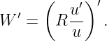
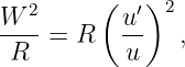
First,
Therefore
Ru2 2 | = R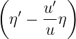 2 | (34)
|
| = R(η′)2 − 2R ηη′ + R  2η2. | (35) |
Next,
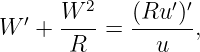
The mixed terms cancel when the two expressions are added. The remaining coefficient of η2
is
But
where the Jacobi equation was used in the last step. This proves the identity.
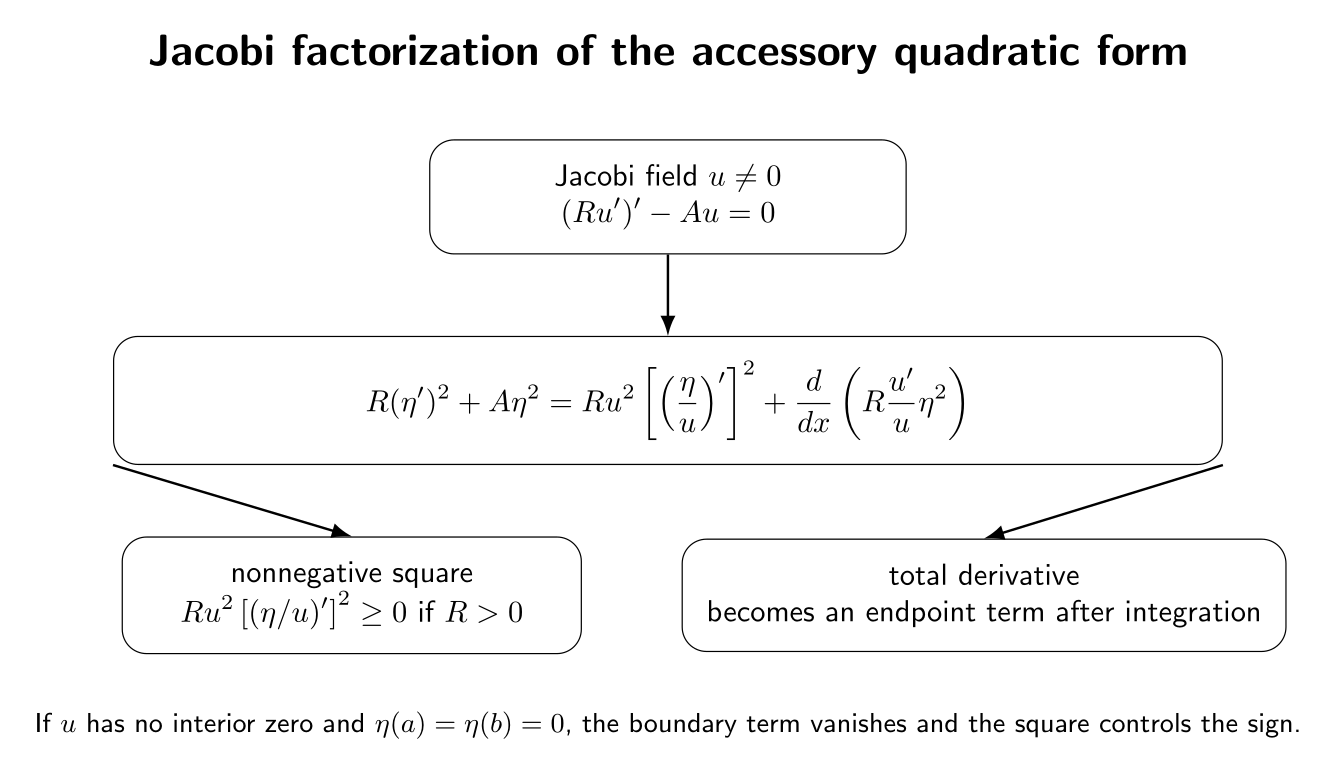
Figure. Jacobi’s factorization rewrites the accessory quadratic form as a manifestly
nonnegative square plus a boundary derivative. The argument works wherever the chosen
Jacobi field does not vanish.
8 Why absence of conjugate points implies positivity
Assume the strengthened Legendre condition
and suppose the distinguished Jacobi field from a has no zero on
Because the normalized field satisfies u(a) = 0, the ratio u′∕u is singular at a. A clean proof
therefore applies the factorization first on
and then lets 𝜀 → 0+.
For a fixed-endpoint variation, the boundary term vanishes at b because
The limiting contribution at a also vanishes for sufficiently regular admissible variations with
η(a) = 0. Hence
Under the regular classical hypotheses, if no conjugate point occurs in (a,b], this representation
yields strict positivity for every nonzero admissible variation.
The key point is that the strengthened Legendre condition supplies
while the absence of conjugate points supplies a Jacobi field u that does not vanish inside the
interval. Both are needed.
9 What happens at the first conjugate point?
Let c1 be the first conjugate point to a. Then there is a nontrivial Jacobi field u satisfying
Multiply the Jacobi equation
by u and integrate from a to c1:
Integrating the first term by parts gives
Since u vanishes at both endpoints,
Thus, if the terminal point b is exactly the first conjugate point,
the second variation has a nontrivial null direction. Strict positivity is lost.
This distinction is important:
- If b < c1, the second variation is positive definite under the regular Jacobi hypotheses.
- If b = c1, a nonzero Jacobi field gives δ2J = 0; a non-strict minimum may still be
possible.
- If b > c1, the quadratic form acquires a negative direction; a weak local minimum is
impossible under the classical regular hypotheses.
The endpoint case is therefore not the same as having a conjugate point strictly inside
(a,b).
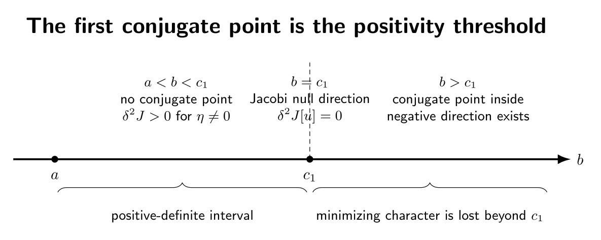
Figure. The first conjugate point marks the threshold. Before it, the accessory quadratic
form is positive definite; at it, a null Jacobi direction appears; beyond it, negative
directions occur.
10 Jacobi’s necessary condition for a minimum
A classical form of Jacobi’s necessary condition can now be stated.
theorem (Jacobi necessary condition, regular scalar case). Suppose y∗ is a sufficiently
smooth weak local minimizer of
with fixed endpoints, and suppose the strengthened Legendre condition
holds along y∗. Then no point of the open interval
can be conjugate to a along y∗.
If b itself is conjugate to a, strict positivity of the second variation fails. Additional information is
needed to decide whether a non-strict minimum remains.
This theorem is a genuinely global-in-the-interval condition. It cannot be obtained by inspecting
Fy′y′ at one point.
11 A Sturm–Liouville viewpoint
Define the differential operator
With fixed endpoints,
integration by parts gives
The Jacobi equation is exactly the zero-eigenvalue equation
More generally, consider the Sturm–Liouville eigenvalue problem
The sign of the smallest eigenvalue controls the sign of the quadratic form:
for every nonzero admissible variation,
and
The first conjugate endpoint is therefore the interval length at which the lowest Dirichlet
eigenvalue reaches zero.
12 Constant coefficients: the three basic cases
Suppose
The Jacobi equation becomes
Three qualitatively different behaviors occur.
12.1 Case 1: A > 0
Then
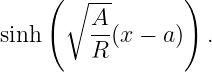
and the distinguished solution is proportional to
It has no zero after a, so there is no finite conjugate point.
12.2 Case 2: A = 0
Then
and the distinguished solution is
Again there is no later zero.
12.3 Case 3: A < 0
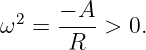
Write
Then
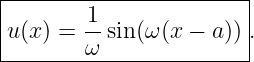
and the normalized solution is
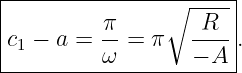
Its first later zero occurs at
This oscillatory case is the model for the harmonic-oscillator action.
13 Worked example: harmonic-oscillator action
Consider
with fixed endpoints
The zero path
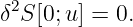
is stationary. Since the action is already quadratic,
Hence
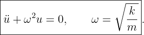
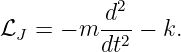
The Jacobi equation is
or
With
we obtain
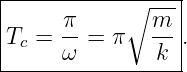
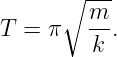
The conjugate times are
The first is
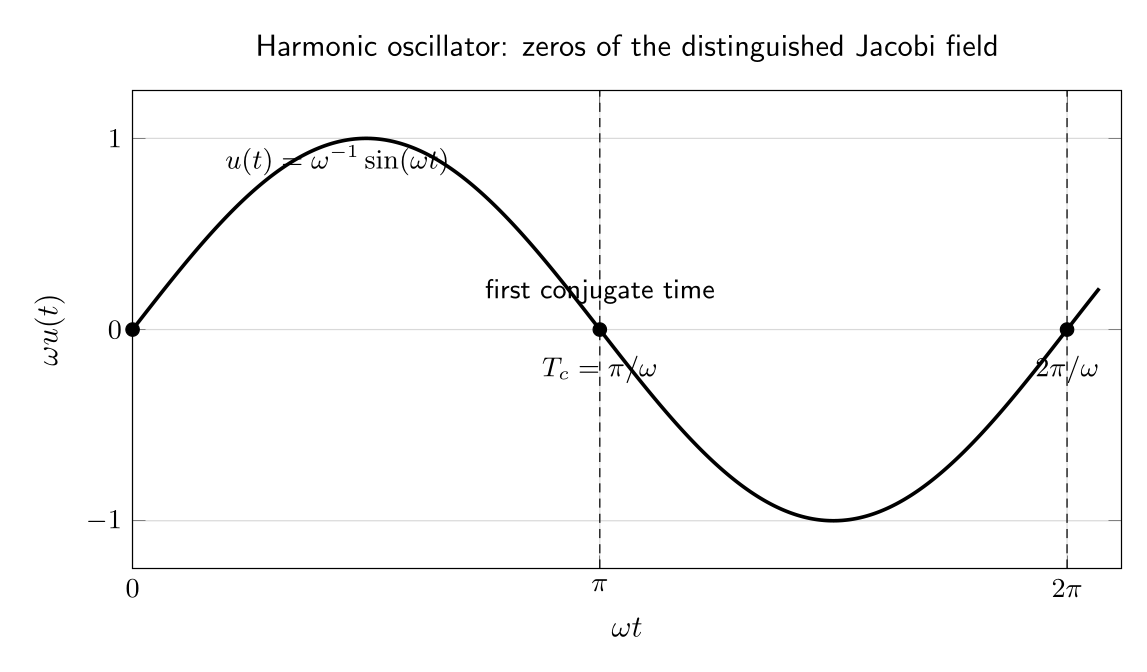
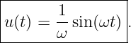
Figure. The distinguished Jacobi field for the harmonic oscillator oscillates and vanishes
at integer multiples of π∕ω. The first later zero is the first conjugate time.
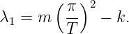
13.1 Short intervals: 0 < T < Tc
No conjugate point lies in (0,T]. Under m > 0, Jacobi’s factorization gives
for every nonzero admissible η. The stationary path is therefore positive to second order.
13.2 Threshold interval: T = Tc
The Jacobi field itself is admissible because
For this nonzero direction,
In fact, because the action is exactly quadratic,
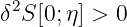
for every amplitude 𝜖. Thus q = 0 is not a strict minimizer, but the appearance of a null direction
at the endpoint does not by itself create a negative direction.
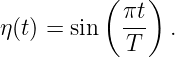
13.3 Long intervals: T > Tc
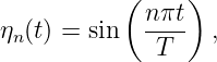
Choose the admissible trial direction
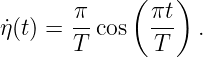
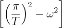
Then
Using
we find
| δ2S[0; η] | =   2 −  | (91)
|
| =   . | (92) |
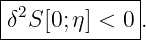
If
then
The stationary path has lost minimizing character.
14 Spectral interpretation of the oscillator threshold
For the harmonic oscillator,
The Dirichlet eigenfunctions on [0,T] are
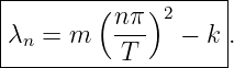
with eigenvalues
The first eigenvalue is
It changes sign exactly when
Thus the first conjugate time and the zero crossing of the lowest eigenvalue are the same event
viewed from two complementary perspectives.
15 A Wronskian identity
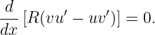
Let u and v be two Jacobi fields satisfying
Multiply the first equation by v, the second by u, and subtract. The Auv terms cancel:
This is
Therefore
This weighted Wronskian identity is the one-dimensional analogue of a conserved symplectic
pairing between neighboring solutions. It is also useful when comparing Jacobi fields and proving
uniqueness properties of their zeros.
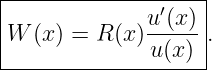
16 Riccati form of the Jacobi equation
Where a Jacobi field u is nonzero, define
Differentiate:
Using
and the identity used in the Jacobi factorization,
so the Jacobi equation gives
This is a scalar Riccati equation. Riccati equations later reappear in optimal control,
linear-quadratic regulation, estimation, and stability theory. Here the singularity of W when u
crosses zero is another way to detect a conjugate point.
17 Geometric preview: conjugate points on a sphere
The language of “Jacobi fields” is especially natural in Differential Geometry. Along a geodesic, a
Jacobi field measures the infinitesimal separation of neighboring geodesics.
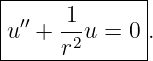
For a sphere of radius r, the Normal Jacobi equation along a unit-speed great circle
is
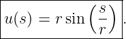
With
we obtain
The first later zero occurs at
That point is the antipode of the starting point. Great circles leaving one point in slightly different
directions reconverge at the antipode. The antipode is therefore conjugate to the starting
point.
This example previews the geodesic material developed later in the series: conjugate
points express a loss of local minimizing behavior caused by the focusing of neighboring
geodesics.
18 What Jacobi’s condition does and does not prove
It is important to separate several logical statements.
18.1 Legendre
The condition
is a local pointwise necessary condition for a weak minimum.
18.2 Jacobi
The absence of conjugate points is an interval-wide necessary condition. Under the
strengthened Legendre condition and standard regularity assumptions, absence of conjugate
points through the terminal endpoint also gives positivity of the accessory quadratic
form.
18.3 Still not the whole story
Even a positive second variation is fundamentally a local quadratic statement. Establishing a
strong minimum, a global minimum, or sufficiency under broad hypotheses requires additional
tools. CV13 develops strengthened Legendre, Weierstrass-type excess conditions, and the
distinction between weak and strong extrema.
19 Common mistakes
- Confusing the original Euler–Lagrange equation with the Jacobi equation.
The first determines stationary candidates; the second governs infinitesimal
perturbations about a stationary candidate.
- Using the wrong coefficients. The Jacobi equation uses the reduced
second-variation coefficients A = Fyy − dFyy′∕dx and R = Fy′y′ evaluated along y∗.
They are not arbitrary coefficients from the original integrand.
- Forgetting that R > 0 is part of the regular Jacobi theory. If R vanishes or
changes sign, the classical argument requires modification.
- Calling every zero a conjugate point without fixing the left endpoint.
Conjugacy is relative to a starting point; one requires a nontrivial Jacobi solution that
vanishes at both locations.
- Treating b = c1 the same as c1 < b. At the first conjugate endpoint there is a null
direction; beyond it a negative direction appears.
- Assuming no conjugate points proves a global minimum. The Jacobi criterion
controls the second variation locally around a stationary extremal.
- Forgetting admissibility. Jacobi fields used as test directions must satisfy the
appropriate linearized endpoint or constraint conditions.
- Ignoring the interval. The same integrand and same extremal can be minimizing on
a short interval and fail to minimize on a longer interval.
- Using the Riccati transform through a zero of u. The quantity u′∕u becomes
singular exactly at a conjugate point.
20 A compact Jacobi workflow
For a regular fixed-endpoint scalar problem:
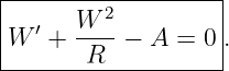
- Find a stationary extremal y∗ from the original Euler–Lagrange equation.
- Compute the reduced second-variation coefficients
- Check the strengthened Legendre condition R > 0 if you intend to use the regular Jacobi
test.
- Form the Jacobi equation
- Solve the normalized initial-value problem
- Locate the first later zero c1.
- Compare b with c1:
- Remember that this is still local classification information; proceed to sufficiency theory when
stronger conclusions are needed.
21 Historical perspective
Euler and Lagrange had established the differential equation now called the Euler–Lagrange
equation, and Legendre had found a second-order sign condition. Yet those results did not fully
decide whether a stationary curve was actually minimizing over an entire interval.
Jacobi addressed this gap in 1837 [7]. His paper, “Zur Theorie der Variations-Rechnung und der
Differential-Gleichungen,” used the accessory equation to make the interval length part of the
classification problem and supplied the precursor of the modern conjugate-point criterion. Classical
developments of the theory can be found in Bliss and Bolza [5, 6].
The conceptual advance can be summarized as
Jacobi’s equation supplies the missing interval-wide information.
22 What CV13 adds
CV11 and CV12 have now developed the local second-order theory:
CV13 turns to stronger sufficiency questions. It distinguishes weak and strong minima, introduces
the Weierstrass excess function, and explains why controlling only infinitesimal slope changes is not
enough for a strong minimum.
Summary
For a stationary extremal, write the reduced second variation as
Its Euler–Lagrange equation is the Jacobi accessory equation
A point c > a is conjugate to a if a nontrivial Jacobi field vanishes at both a and c. Under the
regular strengthened-Legendre hypotheses, the first conjugate point marks the loss of strict
positivity of the second variation:
Jacobi’s factorization
explains why the absence of zeros matters. The harmonic oscillator provides the model example: its
first conjugate time is
exactly the threshold at which the lowest eigenvalue of the second-variation operator crosses
zero.
References
[1] I. M. Gelfand and S. V. Fomin, Calculus of Variations, Dover Publications, 2000.
[2] Bruce van Brunt, The Calculus of Variations, Springer, 2004.
[3] Hans Sagan, Introduction to the Calculus of Variations, Dover Publications, 1992.
[4] Robert Weinstock, Calculus of Variations with Applications to Physics and
Engineering, Dover Publications, 1974.
[5] Gilbert Ames Bliss, Lectures on the Calculus of Variations, University of Chicago
Press, 1946.
[6] Oskar Bolza, Lectures on the Calculus of Variations, University of Chicago Press,
1904.
[7] C. G. J. Jacobi, “Zur Theorie der Variations-Rechnung
und der Differential-Gleichungen,” Journal für die reine und angewandte Mathematik,
17 (1837), 68–82.


























![(a,b].](https://images.physicslibrary.org/cache/objects/1514/make4ht/CalculusOfVariationsTheJacobiEquationAndConjugatePoints46x.png)