|
|
|
|||||||
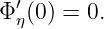
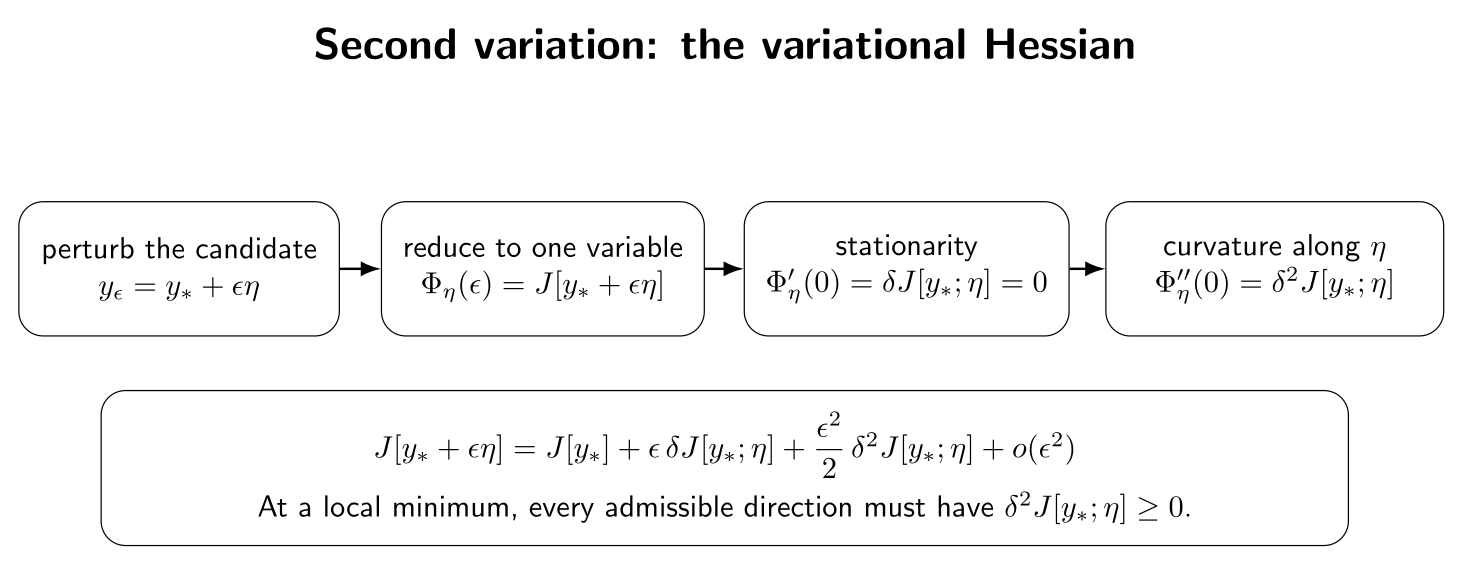
At a stationary function y∗,
The sign of
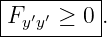
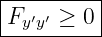
then gives the first classification information in the direction η. The most immediate pointwise consequence is the Legendre necessary condition. For a weak local minimum of a first-order functional, the integrand must satisfy
along the minimizing extremal. This condition is necessary but, crucially, it is not sufficient. The distinction leads directly to the Jacobi equation and conjugate points in CV12. Standard treatments include [1, 2, 3, 4, 5, 6].
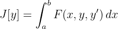
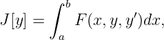
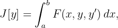
1 From the first variation to the second variationConsider the fixed-endpoint functional
with admissible perturbations
where
Define
The first variation is
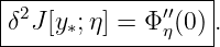
We now define the second variation by
With this convention, the Taylor expansion is
Some books define the “second variation” as the coefficient of 𝜖2 rather than the second derivative itself. That convention differs by a factor of 2. Throughout this series, δ2J means the actual second derivative with respect to 𝜖.
Figure. The second variation is the ordinary second derivative of the scalar slice Φη(𝜖) = J[y∗ + 𝜖η]. At a stationary function the linear term vanishes, so the quadratic term gives the first local classification information.
2 Deriving the second-variation formulaAssume F is C2 in (y,y′) near the candidate. Along the perturbed curve,
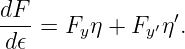
Differentiate once with respect to 𝜖:
Differentiate again. Since η and η′ do not depend on 𝜖,
where equality of the mixed partial derivatives was used. Evaluating at 𝜖 = 0 gives
Every derivative of F in this expression is evaluated along the candidate extremal
The second variation is therefore a quadratic functional in the perturbation η.
3 The bilinear Hessian formIn finite dimensions, the Hessian is naturally bilinear. The same structure exists here. For two admissible directions η and ξ, define
A direct calculation gives
The ordinary second variation is the diagonal case
This is the variational analogue of
for a finite-dimensional Hessian matrix H.
4 Necessary sign condition at a local extremumSuppose y∗ is a weak local minimum. Fix any admissible direction η. For sufficiently small 𝜖,
Equivalently,
Thus the ordinary one-variable function Φη has a local minimum at 𝜖 = 0. Therefore
and
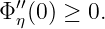
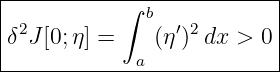
Hence every weak local minimum must satisfy
Likewise, a weak local maximum must satisfy
for every admissible direction. This is necessary, not automatically sufficient.
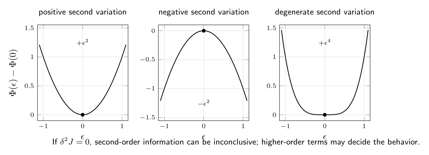
5 Three possible scalar slicesOnce δJ = 0, the second variation plays the same role as the second derivative in ordinary calculus. But a zero second variation can be inconclusive.
Figure. A positive quadratic term suggests minimum behavior along a direction, a negative term suggests maximum behavior, and a vanishing second variation can leave the decision to higher-order terms. The quartic slice +𝜖4 has a strict minimum even though its second derivative at the origin is zero.
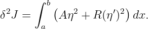
6 Removing the mixed termFor fixed endpoint variations, the mixed term can be rewritten by integration by parts. Introduce
Then
Since
we have
Because η(a) = η(b) = 0, the boundary term vanishes. Thus, when the coefficients are smooth enough,
with
This reduced quadratic functional is often called the accessory functional. It is the starting point for Jacobi’s theory in CV12.
7 The Legendre necessary conditionWe can now derive a pointwise condition from the requirement that the second variation be nonnegative in every localized direction.
7.1 The theoremLegendre necessary condition. Let
with F ∈ C2 in a neighborhood of a weak local minimizing extremal y ∗. Then
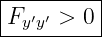
for every x ∈ [a,b]. For a weak local maximum, the inequality is reversed.
7.2 Proof by a localized perturbationSuppose, for contradiction, that at some interior point x0,
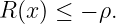
By continuity, there exist ρ > 0 and a small neighborhood of x0 in which
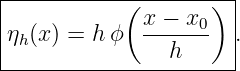
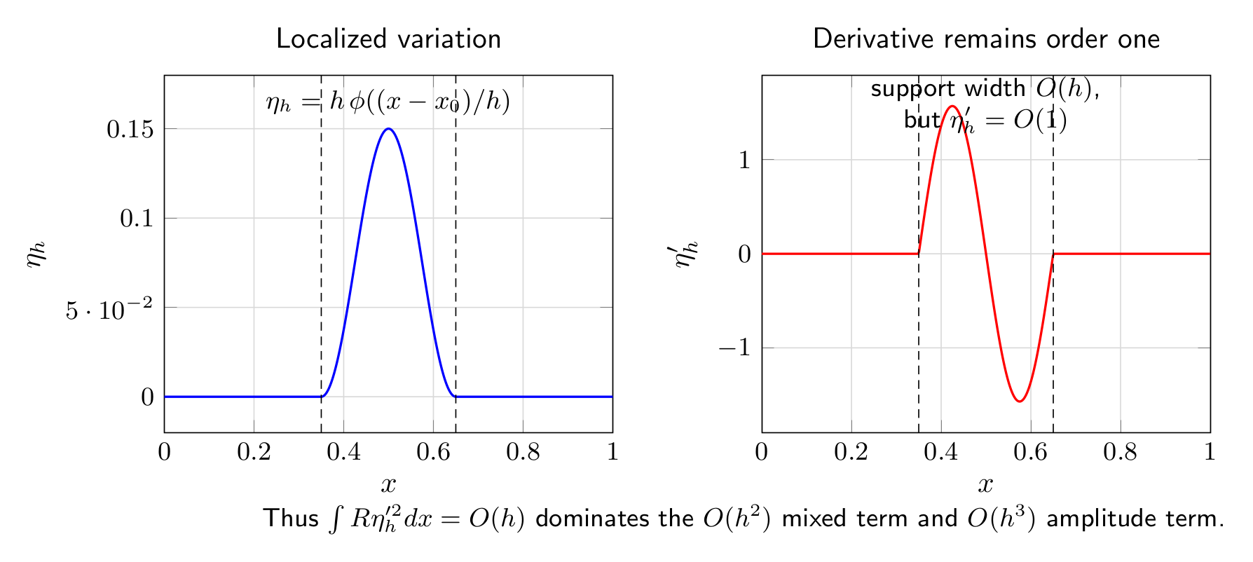
Choose a nonzero smooth bump ϕ ∈ Cc∞(−1, 1) and define the localized variation
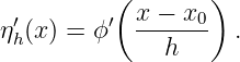
Its support has width O(h), its amplitude is O(h), and
This derivative does not shrink in amplitude as h → 0.
Figure. Legendre localization. The perturbation amplitude shrinks with h, but its derivative remains order one. Consequently the Fy′y′(η′)2 contribution is order h and dominates the lower-order amplitude and mixed terms as the support collapses. Use the unreduced second-variation formula
Set
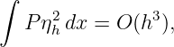
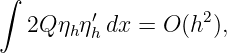
The three contributions scale as
while
The last term is strictly negative and of order h. Therefore, for sufficiently small h,
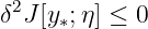
This contradicts the necessary condition δ2J ≥ 0 for a weak local minimum. Hence
The endpoint values follow by continuity from the interior result. □
8 Why the Legendre condition is localThe proof explains the physics of the theorem. A very narrow perturbation can have tiny displacement but a finite slope perturbation. Therefore, if the integrand is locally concave in y′, a sufficiently localized ripple immediately lowers the functional. The Legendre condition tests only this highest-gradient curvature:
It does not test the full competition between the η2 and (η′)2 terms over a finite interval. That missing global-in-x information is exactly why the Legendre condition is not sufficient.
9 The strengthened Legendre conditionThe strengthened Legendre condition for a minimum is
along the extremal, often strengthened further to a uniform bound
For a maximum, the corresponding strengthened condition is
The strengthened condition is not necessary for every minimum. A minimizing functional can be degenerate and have Fy′y′ = 0 at some or all points. Its importance is that it supplies coercivity in the derivative term and becomes a key ingredient in stronger sufficient-condition theorems.
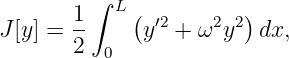
10 Example: positive quadratic energyConsider
with
The zero function is stationary. Here
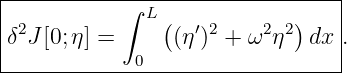
Thus
For every nonzero admissible η this is positive. In fact, because the original functional itself is already a nonnegative quadratic form,
so y = 0 is the unique global minimizer. This is an unusually clean case: stationarity, positive second variation, and direct global minimality all agree.
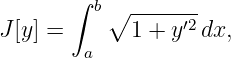
11 Example: arc length near a straight lineFor
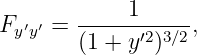
consider the horizontal stationary line y∗ = 0. Since
we have along y∗ = 0
Also Fyy = Fyy′ = 0, so
for every nonzero fixed-endpoint perturbation. This agrees with the geometric fact that the straight segment is the shortest path between its endpoints.
12 Example: the Legendre condition is not sufficientConsider the harmonic-oscillator action
with fixed endpoint values
The stationary solution
satisfies the strengthened Legendre condition. Writing v for the velocity argument dq∕dt of the Lagrangian,
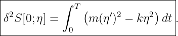
Nevertheless,
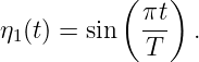
Choose the admissible direction
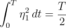
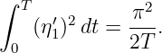
Then
and
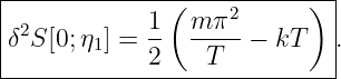
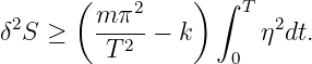
Therefore
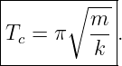
The sign changes at
For T > Tc, this admissible direction has negative second variation even though Lvv = m > 0 everywhere.
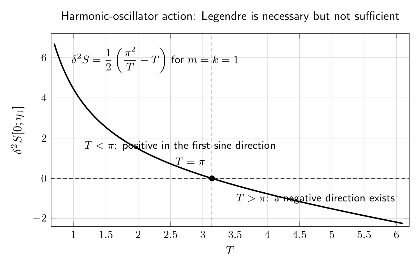
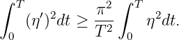
Figure. For m = k = 1, the second variation in the first sine direction changes sign at T = π. The strengthened Legendre condition remains true for every T, so it cannot by itself guarantee a minimum. The Wirtinger inequality sharpens the conclusion. For every fixed-endpoint perturbation,
Hence
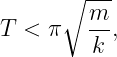
Thus the second variation is positive definite for
degenerate at the critical interval, and indefinite beyond it. CV12 will interpret this threshold in terms of a conjugate point.
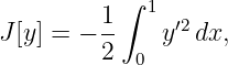
13 Example: violating Legendre gives a maximum directionConsider
with y(0) = y(1) = 0. The zero function is stationary, but
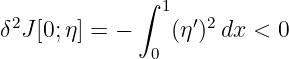
Therefore the Legendre condition for a minimum fails immediately. Indeed,
for every nonzero admissible direction. The zero function is a strict maximum within this quadratic problem.
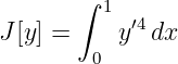
14 Example: a degenerate minimum with zero second variationConsider
with fixed zero endpoints. The zero function is a global minimizer because
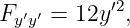
But
so along y∗ = 0,
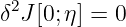
Consequently
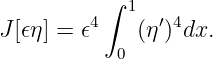
for every direction. The first nonzero change is fourth order:
This example shows why the strengthened Legendre condition is not necessary and why a vanishing second variation is inconclusive rather than evidence against a minimum.
15 The accessory equation and the bridge to JacobiReturn to the reduced second variation
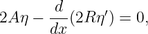
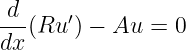
Treat this quadratic expression itself as a new variational functional in η. Its Euler–Lagrange equation is
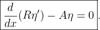
or
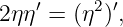
This is the Jacobi accessory equation. Nontrivial solutions satisfying suitable endpoint conditions are called Jacobi fields in the one-dimensional setting. The key new phenomenon is that even if
the Aη2 term can still make the quadratic form lose positivity over a sufficiently long interval. The first location where a nontrivial Jacobi field vanishes again is a conjugate point. CV12 develops this criterion in detail.
16 Historical perspectiveThe second variation is historically important because it exposed the limits of merely solving Euler–Lagrange. Legendre developed an early second-order necessary sign condition involving the coefficient now written Fy′y′. Later work, especially by Jacobi, showed that this local sign test does not completely classify an extremal; interval-wide information encoded by the accessory equation and conjugate points is also required. Classical historical and technical discussions can be found in [5, 6, 4]. This progression mirrors ordinary calculus but with an important infinite-dimensional twist:
17 Common mistakes
18 A compact second-variation workflowFor a first-order fixed-endpoint problem, use the following sequence.
19 What CV12 addsCV11 has established the variational analogue of the Hessian and extracted the Legendre necessary condition. The harmonic-oscillator example showed the central limitation: even a strictly positive Fy′y′ does not prevent the second variation from becoming negative because of the lower-order term. CV12 studies the accessory equation
and introduces conjugate points. This produces a genuinely interval-dependent test for the loss of minimizing character and explains the critical-time behavior seen in mechanical action problems.
SummaryFor a stationary extremal y∗ of
the second variation is
At a weak local minimum,
Localized variations then force the Legendre necessary condition
After integration by parts, the quadratic form can be written as
The Legendre condition is necessary but not sufficient. The full sign of the second variation depends on the interval and on the interaction of both coefficients. That remaining problem leads directly to Jacobi’s equation and conjugate points.
References
[1] I. M. Gelfand and S. V. Fomin, Calculus of Variations, Dover Publications, 2000. [2] Bruce van Brunt, The Calculus of Variations, Springer, 2004. [3] Hans Sagan, Introduction to the Calculus of Variations, Dover Publications, 1992. [4] Robert Weinstock, Calculus of Variations with Applications to Physics and Engineering, Dover Publications, 1974. [5] Gilbert Ames Bliss, Lectures on the Calculus of Variations, University of Chicago Press, 1946. [6] Oskar Bolza, Lectures on the Calculus of Variations, University of Chicago Press, 1904. [7] Cornelius Lanczos, The Variational Principles of Mechanics, Dover Publications, 1986. "Calculus of Variations: The Second Variation and the Legendre Condition" is owned by bloftin.
This object's parent.
Cross-references: force, Taylor series, work, Jacobi fields, accessory equation, Lagrangian, velocity, displacement, theorem, formula, amplitude, boundary, matrix, dimensions, CV12, conjugate points, Jacobi equation, scalar, functions There are 6 references to this object. This is version 1 of Calculus of Variations: The Second Variation and the Legendre Condition, born on 2026-10-20. Object id is 1512, canonical name is CalculusOfVariationsTheSecondVariationAndTheLegendreCondition. Accessed 3 times total. Classification:
|
|
|
|
Pending Errata and AddendaNone.
|
DiscussionNo messages.
|
Interact |
















![]](https://images.physicslibrary.org/cache/objects/1512/make4ht/CalculusOfVariationsTheSecondVariationAndTheLegendreCondition20x.png)