Calculus of Variations: Functionals, Admissible Functions, and Extrema
The calculus of variations does not ask merely for a number that minimizes a function. It asks for
an entire function, curve, field, or trajectory that optimizes a scalar quantity. Before differentiating
a functional, one must therefore answer three questions:
- What objects is the functional allowed to act on?
- Which of those objects are physically and mathematically admissible?
- What does it mean for two admissible functions to be “near” one another?
The third question is easy to overlook. In ordinary single-variable calculus, closeness is inherited
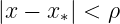
from the usual distance |x−x∗|. In a function space there are many inequivalent ways to measure
distance. Two curves can be very close in height while having very different slopes. Consequently,
the phrase “local minimum” is incomplete until the relevant neighborhood of functions has been
specified.
This entry develops that foundation. It introduces admissible classes, function spaces, norms,
relative and global extrema, and the classical distinction between weak and strong extrema. CV02
will then use these ideas to define variations and the first variation.
1 Learning objectives
After this entry, the reader should be able to
- identify the domain of a functional and distinguish it from the domain of an ordinary
function;
- construct an admissible class from smoothness, endpoint, integral, or inequality
constraints;
- explain why an admissible class need not be a vector space;
- distinguish C0, C1, and C2 regularity at an introductory level;
- define the uniform C0 norm and a standard C1 norm;
- explain why a local extremum is defined relative to both an admissible set and a notion
of neighborhood;
- distinguish global, local, weak, and strong minima and maxima;
- prove that a global minimum is a strong local minimum and that a strong local
minimum is a weak local minimum in the classical setting;
- understand by explicit example how a weak minimum can fail to be a strong minimum;
and
- distinguish attainment of a minimum from the mere existence of an infimum.
2 A functional includes its domain
A functional is a mapping
where 𝒜 is the domain of admissible objects. In the classical first-order problem,
𝒜 is usually a class of sufficiently smooth real-valued functions on [a,b] satisfying specified
constraints.
It is mathematically incomplete to specify only the formula for J[y] and leave 𝒜 implicit. The same
integral expression can define different optimization problems on different admissible
classes.
For example, consider
One possible domain is
Another is
The formula for J is identical, but the optimization problems are not. The first class forces the
curve to connect (0, 0) to (1, 1); the second forces it to return to zero.
3 Admissible functions and admissible classes
An admissible function is a function permitted by all constraints of the variational problem. The
collection of all such functions is the admissible class 𝒜.
The constraints defining 𝒜 can come from mathematics, physics, or both.
3.1 Regularity constraints
The integrand may require derivatives to exist. If
then a classical treatment commonly assumes y ∈ C1([a,b]). If
then C2 regularity may be assumed in an elementary treatment.
Later analysis often weakens these assumptions. For example, finite-energy problems naturally lead
to Sobolev spaces in which derivatives may exist only in a weak sense. The present course begins
with classical Ck spaces so the variational logic is visible before the functional-analytic
generalization is introduced.
3.2 Endpoint constraints
A fixed-endpoint class has the form
The endpoint conditions are not decorative boundary data appended after the variational
calculation. They determine which comparison curves are allowed and, in CV02, which variations
are allowed.
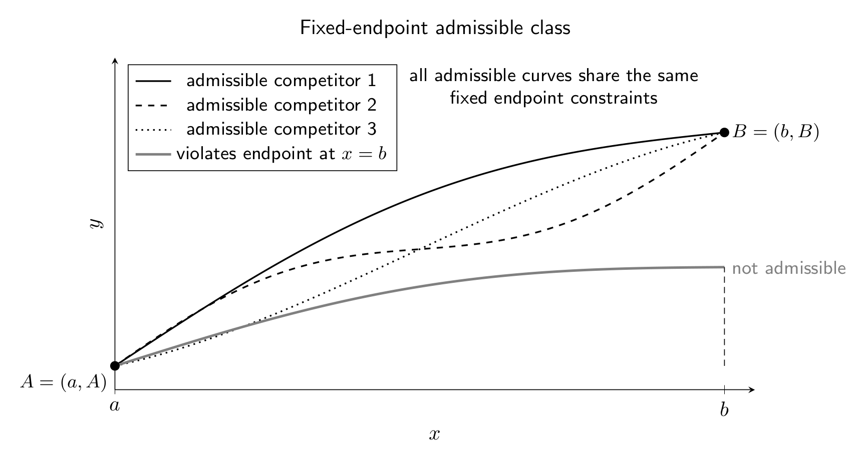
Figure. Several curves can belong to the same fixed-endpoint admissible class even though
their interior shapes differ substantially. A curve that violates an endpoint condition is not
a competitor at all.
3.3 Periodic and mixed constraints
A periodic class might require
A mixed problem might fix one endpoint but leave the other free:
Such changes alter the endpoint terms that survive integration by parts. Natural boundary
conditions and transversality conditions are developed in CV05.
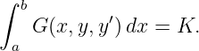
3.4 Integral constraints
An isoperimetric problem may impose an additional condition such as
The admissible class is then restricted to functions satisfying both the endpoint conditions and the
integral constraint. CV09 develops the variational Lagrange-multiplier method for this
situation.
3.5 Inequality and obstacle constraints
A physical path may be forbidden from entering part of the domain. An obstacle problem can
contain a condition such as
This is an important reminder that an admissible class need not be a vector space. If y1 and y2 are
admissible, an arbitrary linear combination
need not satisfy the same endpoint, integral, or inequality constraints.
4 Function spaces used in the classical theory
To speak about neighborhoods of functions, we first need a space in which the functions
live.
4.1 The space C0([a,b])
The notation
denotes the continuous real-valued functions on [a,b].
A natural measure of size is the uniform or supremum norm
For two functions y and z, the induced distance is
Thus y and z are close in C0 if their graphs remain vertically close at every point.
4.2 The space C1([a,b])
The space C1([a,b]) contains functions whose first derivatives exist and are continuous. For the
present series, define
Then
requires both the functions and their first derivatives to be close.
Another common convention is
These two formulas define equivalent norms on C1([a,b]) and therefore the same notion of local
convergence. The max convention is used here because it makes the inclusion of neighborhoods
especially transparent.
4.3 The space C2([a,b])
Similarly, C2([a,b]) contains functions with continuous first and second derivatives. A
corresponding norm can be defined by
The higher the norm order, the more derivative information is controlled by a small
neighborhood.
5 Neighborhoods of functions
Let y∗ be a candidate function. Its open C0 neighborhood of radius ρ > 0 is
Its open C1 neighborhood is
Because
we have
This inclusion is the geometric reason a strong variational minimum is a stronger property than a
weak minimum, despite the initially counterintuitive terminology.
A C1 neighborhood is smaller because it excludes curves whose heights are close but whose slopes
change rapidly. A C0 neighborhood is larger because it allows such highly oscillatory
competitors.
6 Global extrema
Let J : 𝒜→ ℝ.
6.1 Global minimum
A function y∗ ∈𝒜 is a global minimum or global minimizer if
It is a strict global minimum if
A global maximum is defined by reversing the inequalities.
The defining feature is that a global optimum is compared with the entire admissible class. No
notion of distance is needed.
7 Local or relative extrema
A local minimum compares y∗ only with admissible functions in a neighborhood of y∗. The
mathematically precise statement requires both an admissible set and a distance or
topology.
Let d be a distance on the ambient function space. The function y∗ ∈𝒜 is a local minimum relative
to 𝒜 if there exists ρ > 0 such that
for every
The word relative means relative to the admissible set 𝒜. It does not mean weak or strong. Weak
and strong extrema are two different ways of choosing the neighborhood in which the relative
comparison is made.
This distinction mirrors finite-dimensional constrained optimization. If a point is constrained to a
surface, “local” means local among points on that surface, not among all points of the surrounding
space.
7.1 Why local extrema require a topology
In ordinary calculus, the statement
has an obvious meaning. For functions there is no single universally correct analogue. One
may control values, derivatives, integral averages, or other properties. Different choices
generate different neighborhoods and therefore potentially different notions of local
optimality.
The classical first-order calculus of variations gives special names to two important choices: weak
extrema and strong extrema.
8 Weak local extrema
For a first-order functional on a C1 admissible class, y
∗ is a weak local minimum if there exists
ρ > 0 such that
for every admissible y satisfying
Equivalently, both
and
must hold under the max-norm convention.
Thus weak minimality tests the candidate against curves that are close in both position and
slope.
A weak local maximum is defined by reversing the inequality.
9 Strong local extrema
The function y∗ is a strong local minimum if there exists ρ > 0 such that
for every admissible y satisfying only
The derivatives of y and y∗ are not required to be close.
This means a strong minimum must survive comparison with a larger set of nearby
curves, including small-amplitude, high-frequency oscillations that can have large slope
changes.
The term “strong” therefore refers to the strength of the optimality claim, not to a stronger
closeness requirement.
10 Hierarchy of minimum concepts
The classical implications are
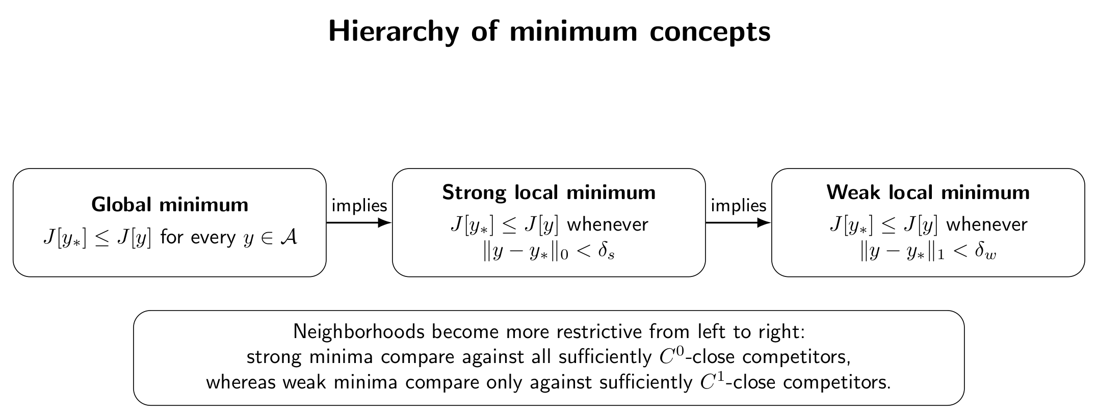
Figure. A global minimum is compared with every admissible function. A strong local
minimum is compared with every sufficiently C0-close admissible function. A weak local
minimum is compared only with sufficiently C1-close admissible functions.
10.1 Proposition: global implies strong, and strong implies weak
proposition. Let J be defined on an admissible class 𝒜⊂ C1([a,b]). Using the norms defined
above:
- every global minimum is a strong local minimum;
- every strong local minimum is a weak local minimum.
Proof. If y∗ is a global minimum, then
for every y ∈𝒜. Therefore the same inequality certainly holds for the smaller collection of
admissible functions satisfying ∥y − y∗∥0 < ρ, for any ρ > 0. Hence y∗ is a strong local
minimum.
Now suppose y∗ is a strong local minimum. Then for some ρ > 0,
for every admissible y in N0(y∗; ρ). But
Therefore the same inequality holds for every admissible y in the smaller C1 neighborhood
N1(y∗; ρ). Hence y∗ is a weak local minimum. □
The converses are false in general. The next example explicitly proves the failure of the
strong-to-weak converse.
11 Example: a global minimizer proved without Euler–Lagrange
Consider
on
We claim that
is the unique global minimizer.
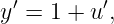
Every admissible function can be written as
where
Then
and therefore
Expanding,
By the Fundamental theorem of Calculus,
Hence
But
Thus
Equality requires
for every x, and the endpoint conditions then force u = 0. Therefore y∗(x) = x is the unique global
minimizer.
This proof is stronger than a stationarity calculation. It does not merely produce a
necessary differential equation; it directly compares the candidate with every admissible
function.
12 Why weak and strong minima are genuinely different
A curve can be arbitrarily close to another curve in C0 while remaining far away in
C1.
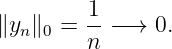
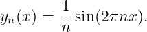
Consider
Then
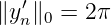
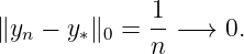
Thus yn → 0 uniformly. However,
so
for every n. The derivatives do not approach zero at all.
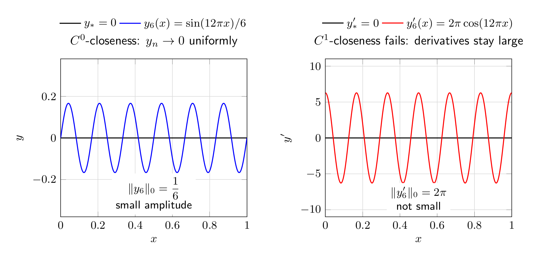
Figure. The functions yn = sin(2πnx)∕n converge uniformly to zero because their
amplitudes shrink as 1∕n, but their derivative amplitudes remain 2π. They become
C0-close without becoming C1-close.
This phenomenon allows a weak minimum to fail to be a strong minimum.
13 Worked counterexample: weak minimum but not strong minimum
Define
on the fixed-endpoint class
Consider the candidate
Its functional value is
13.1 Step 1: prove weak local minimality
Choose any radius ρ satisfying
If
then in particular
Therefore
Integrating gives
Thus y∗ = 0 is a weak local minimum.
13.2 Step 2: construct C0-near curves with lower cost
Use the admissible sequence
Each yn satisfies
and
So every C0 neighborhood of y
∗ contains yn for sufficiently large n.
But
Therefore
Using
and
we obtain
Since
we have
for every n.
Thus arbitrarily C0-close admissible curves have lower functional value. The zero function is
therefore not a strong local minimum.
This example proves concretely that
The failure is caused by high-frequency perturbations: their amplitudes are small, but their slopes
are not.
14 Why the terminology feels reversed at first
It is tempting to think that a “strong neighborhood” should control more quantities than a “weak
neighborhood.” Classical variational terminology uses the words in the opposite logical
sense.
A weak minimum is required to defeat only competitors that are close in both y and y′. That is a
relatively small comparison set.
A strong minimum is required to defeat every competitor whose graph is close in y, even if
its derivative differs greatly. That is a larger comparison set and therefore a stronger
claim.
One useful memory aid is
rather than “strong means more derivatives are close.”
15 Strict local extrema
A weak or strong local minimum is called strict if the inequality is strict for every distinct
admissible competitor in the relevant neighborhood. For example, a strict strong local minimum
satisfies
for every admissible y≠y∗ sufficiently close in C0.
Strictness concerns uniqueness inside the local neighborhood. It is separate from the
weak-versus-strong distinction.
16 Maximum, minimum, and saddle-type behavior
All definitions above have corresponding maximum forms obtained by reversing inequalities.
A stationary function, once stationarity is defined in CV02, need not be a minimum or a
maximum. It may have saddle-type behavior: some admissible perturbations increase the
functional while others decrease it.
The ordinary-calculus analogy remains useful:
is not enough to classify x∗. Likewise, the eventual Euler–Lagrange equation identifies stationary
candidates but does not by itself prove minimum or maximum behavior.
This is why the series later develops the second variation, Legendre condition, Jacobi equation,
conjugate points, and Weierstrass condition.
17 Extremal versus minimizer: terminology discipline
Classical texts sometimes use the word extremal in more than one way. It may mean an actual
function giving a local extremum, or it may mean a solution of the Euler–Lagrange equation even
before minimum or maximum character has been established.
To avoid that ambiguity, this series uses the following language whenever possible:
- minimizer or maximizer: a function satisfying the actual optimization inequality;
- stationary function: a function whose first variation vanishes for every admissible
first-order variation;
- Euler–Lagrange extremal: used only when referring to the common classical
terminology for a solution of the Euler–Lagrange equation.
Thus a later statement that “y∗ is stationary” should never be silently upgraded to “y∗ minimizes
J.”
18 A minimum value need not be attained
Optimization contains another distinction that is independent of weak and strong local behavior: a
functional can have an infimum without possessing a minimizer.
Consider the admissible class of positive constant functions on [0, 1],
and the functional
For yc,
The values can be made arbitrarily close to zero by choosing c small, so
However, c = 0 is excluded from 𝒜. No admissible function attains the value zero. Therefore no
global minimizer exists.
A minimizing sequence is
for which
The limiting function y = 0 lies on the boundary of the admissible class but not inside
it.
This simple example foreshadows a major branch of modern variational analysis: existence theory.
The direct method of the calculus of variations studies conditions such as compactness, coercivity,
closedness of the admissible set, and lower semicontinuity that prevent a minimizing sequence from
escaping without converging to an admissible minimizer.
19 The admissible set is part of the physics
In physical applications, the admissible class encodes what trajectories are physically possible
before any optimization principle is applied.
19.1 Classical mechanics
Hamilton’s principle uses histories q(t) connecting prescribed endpoint configurations. In its
standard fixed-endpoint form,
The comparison histories are not required to satisfy the equations of motion. They are
kinematically admissible alternatives used to test stationarity of the action.
19.2 Geometrical optics
A ray path must connect source and observation points and remain within the physical optical
medium. Interfaces or forbidden regions alter the admissible set and can generate additional corner
or transversality conditions.
19.3 Elasticity and field theory
Boundary conditions can prescribe displacement, traction, field values, or periodicity. The natural
function space is often selected by finiteness of the physical energy rather than by an arbitrary
desire for smoothness.
For example, an energy containing
suggests controlling first derivatives in an integral sense. This is one of the reasons Sobolev spaces
become natural in continuum and field theories.
20 Neighborhood choice and physical perturbations
The weak-versus-strong distinction has a physical interpretation. A weak neighborhood excludes
perturbations with large slope or velocity changes. A strong neighborhood can include
high-frequency, small-amplitude perturbations.
Whether those perturbations are physically meaningful depends on the model. A continuum model
that ignores small-scale microstructure may cease to be valid for arbitrarily rapid oscillations.
Conversely, if the physical theory does permit such perturbations, a proposed minimum should
survive them.
The mathematical topology therefore encodes a statement about which kinds of nearby behavior
are being tested.
21 Common misconceptions
21.1 Misconception 1: the formula for J defines the whole problem
It does not. The admissible class, regularity, and constraints are part of the definition.
21.2 Misconception 2: every admissible class is a vector space
Endpoint, integral, and inequality constraints can destroy closure under addition and scalar
multiplication.
21.3 Misconception 3: “relative extremum” means weak extremum
It does not. Relative means relative to the admissible set. Weak and strong specify the type of
function-space neighborhood used for local comparison.
21.4 Misconception 4: strong minimum means y′ must also be close
The classical definition is the opposite. Strong minimality controls only the graph distance in C0
and therefore tests against a larger class of nearby curves.
21.5 Misconception 5: a weak minimum is almost the same as a strong one
The oscillatory counterexample in this entry shows that the difference can be fundamental.
Small-amplitude curves can have large derivatives and can reveal directions of decrease invisible
inside a small C1 neighborhood.
21.6 Misconception 6: if the infimum is finite, a minimizer exists
Not necessarily. A minimizing sequence can converge to an object outside the admissible class or
fail to converge in the required topology.
21.7 Misconception 7: solving Euler–Lagrange will prove the minimum
Euler–Lagrange is a stationarity condition. Classification and existence are separate
questions.
22 A compact definition table
For a functional J : 𝒜→ ℝ and candidate y∗ ∈𝒜:
|
|
concept | Definition / comparison set |
|
|
Global minimum | J[y∗] ≤ J[y] for every y ∈𝒜. |
|
|
Local or relative
minimum | J[y∗] ≤ J[y] for admissible y in some neighborhood of y∗. The
neighborhood topology must be specified. |
|
|
Weak local
minimum | Local minimum with respect to a C1-type neighborhood; both
y and y′ are required to be close. |
|
|
Strong local
minimum | Local minimum with respect to a C0-type neighborhood; y is
close, but y′ may differ substantially. |
|
|
Strict minimum | The relevant inequality is strict for every distinct competitor
in the comparison set. |
|
|
Infimum | Greatest lower bound of the attainable functional values; it
need not itself be attained. |
|
|
23 What CV02 adds
The present entry has defined what it means for a function to be locally optimal, but it has not yet
derived a practical necessary condition for such an optimum.
CV02 introduces an admissible perturbation
and converts the functional into an ordinary scalar function of 𝜖,
The first variation will be defined by
The logical bridge will then be the infinite-dimensional analogue of Fermat’s necessary
condition:
If an admissible function is a sufficiently regular local extremum, then the
first-order change must vanish in every admissible direction.
That statement is the beginning of stationarity. CV03 will prove the Fundamental Lemma needed
to turn stationarity into a pointwise equation, and CV04 will derive the Euler–Lagrange
equation.
24 Summary
A variational problem consists of more than an integral formula. It requires an admissible class 𝒜,
a functional J, and a precise notion of comparison.
For classical first-order problems, the most important neighborhood norms are
and
A weak local minimum is tested against sufficiently C1-close curves. A strong local minimum is
tested against the larger set of sufficiently C0-close curves. Consequently,
while the converses need not hold.
The phrase “relative extremum” refers to optimization relative to the admissible set; it is not a
synonym for weak extremum. Finally, even a finite infimum need not be attained, so existence of a
minimizer is logically separate from stationarity and classification.
These definitions supply the topology and optimization language needed for CV02, where nearby
admissible functions become one-parameter variations and the first variation is derived
rigorously.
25 References and further reading
- I. M. Gelfand and S. V. Fomin, Calculus of Variations, Dover Publications.
- R. Weinstock, Calculus of Variations with Applications to Physics and Engineering,
Dover Publications.
- M. Giaquinta and S. Hildebrandt, Calculus of Variations I: The Lagrangian Formalism,
Springer.
- B. Dacorogna, Direct Methods in the Calculus of Variations, Springer.
- C. Lanczos, The Variational Principles of Mechanics, Dover Publications.

![J : 𝒜 → ℝ, y ↦→ J[y],](https://images.physicslibrary.org/cache/objects/1197/make4ht/AdmissibleFunctionsCalculusOfVariationsFunctionals0x.png)
![∫
b ′
J[y] = F (x,y(x),y (x)) dx,
a](https://images.physicslibrary.org/cache/objects/1197/make4ht/AdmissibleFunctionsCalculusOfVariationsFunctionals1x.png)
![∫
1 ′ 2
J[y] = y (x) dx.
0](https://images.physicslibrary.org/cache/objects/1197/make4ht/AdmissibleFunctionsCalculusOfVariationsFunctionals2x.png)
![{ 1 }
𝒜1 = y ∈ C ([0,1]) : y(0) = 0, y(1) = 1 .](https://images.physicslibrary.org/cache/objects/1197/make4ht/AdmissibleFunctionsCalculusOfVariationsFunctionals3x.png)
![{ 1 }
𝒜2 = y ∈ C ([0,1]) : y(0) = y(1) = 0 .](https://images.physicslibrary.org/cache/objects/1197/make4ht/AdmissibleFunctionsCalculusOfVariationsFunctionals4x.png)


![{ }
𝒜 = y ∈ C1([a,b]) : y (a) = A, y(b) = B .](https://images.physicslibrary.org/cache/objects/1197/make4ht/AdmissibleFunctionsCalculusOfVariationsFunctionals7x.png)


![y(x ) ≥ ψ(x) for every x ∈ [a,b].](https://images.physicslibrary.org/cache/objects/1197/make4ht/AdmissibleFunctionsCalculusOfVariationsFunctionals11x.png)

![0
C ([a,b]) = C([a,b])](https://images.physicslibrary.org/cache/objects/1197/make4ht/AdmissibleFunctionsCalculusOfVariationsFunctionals13x.png)
![∥y ∥0 = max |y(x)|.
x∈[a,b]](https://images.physicslibrary.org/cache/objects/1197/make4ht/AdmissibleFunctionsCalculusOfVariationsFunctionals14x.png)
![d (y,z) = ∥y − z∥ = max |y(x) − z(x)|.
0 0 x∈[a,b]](https://images.physicslibrary.org/cache/objects/1197/make4ht/AdmissibleFunctionsCalculusOfVariationsFunctionals15x.png)








![J[y∗] ≤ J [y] for every y ∈ 𝒜.](https://images.physicslibrary.org/cache/objects/1197/make4ht/AdmissibleFunctionsCalculusOfVariationsFunctionals24x.png)
![J[y ] < J[y] for every y ∈ 𝒜, y ⁄= y .
∗ ∗](https://images.physicslibrary.org/cache/objects/1197/make4ht/AdmissibleFunctionsCalculusOfVariationsFunctionals25x.png)
![J[y ] ≤ J[y]
∗](https://images.physicslibrary.org/cache/objects/1197/make4ht/AdmissibleFunctionsCalculusOfVariationsFunctionals26x.png)

![J[y∗] ≤ J[y]](https://images.physicslibrary.org/cache/objects/1197/make4ht/AdmissibleFunctionsCalculusOfVariationsFunctionals29x.png)



![J[y∗] ≤ J[y]](https://images.physicslibrary.org/cache/objects/1197/make4ht/AdmissibleFunctionsCalculusOfVariationsFunctionals33x.png)


![J[y∗] ≤ J[y]](https://images.physicslibrary.org/cache/objects/1197/make4ht/AdmissibleFunctionsCalculusOfVariationsFunctionals36x.png)
![J[y∗] ≤ J[y]](https://images.physicslibrary.org/cache/objects/1197/make4ht/AdmissibleFunctionsCalculusOfVariationsFunctionals37x.png)

![∫ 1
J [y] = y′(x)2 dx
0](https://images.physicslibrary.org/cache/objects/1197/make4ht/AdmissibleFunctionsCalculusOfVariationsFunctionals39x.png)
![𝒜 = {y ∈ C1 ([0, 1]) : y(0) = 0, y(1) = 1}.](https://images.physicslibrary.org/cache/objects/1197/make4ht/AdmissibleFunctionsCalculusOfVariationsFunctionals40x.png)



![∫ 1
J[y] = (1 + u′)2dx.
0](https://images.physicslibrary.org/cache/objects/1197/make4ht/AdmissibleFunctionsCalculusOfVariationsFunctionals45x.png)
![∫ 1 ∫ 1
J [y] = 1 + 2 u′dx + u′2dx.
0 0](https://images.physicslibrary.org/cache/objects/1197/make4ht/AdmissibleFunctionsCalculusOfVariationsFunctionals46x.png)

![∫ 1
J[y] = 1 + u′(x)2dx ≥ 1.
0](https://images.physicslibrary.org/cache/objects/1197/make4ht/AdmissibleFunctionsCalculusOfVariationsFunctionals48x.png)
![∫ 1
J [y ] = 12 dx = 1.
∗ 0](https://images.physicslibrary.org/cache/objects/1197/make4ht/AdmissibleFunctionsCalculusOfVariationsFunctionals49x.png)
![J[y] ≥ J[y∗] for every y ∈ 𝒜.](https://images.physicslibrary.org/cache/objects/1197/make4ht/AdmissibleFunctionsCalculusOfVariationsFunctionals50x.png)



![∫
1( ′ 2 ′ 4)
J[y] = y (x) − y(x) dx
0](https://images.physicslibrary.org/cache/objects/1197/make4ht/AdmissibleFunctionsCalculusOfVariationsFunctionals56x.png)
![{ 1 }
𝒜 = y ∈ C ([0,1]) : y(0) = y (1 ) = 0 .](https://images.physicslibrary.org/cache/objects/1197/make4ht/AdmissibleFunctionsCalculusOfVariationsFunctionals57x.png)
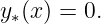
![J[y∗] = 0.](https://images.physicslibrary.org/cache/objects/1197/make4ht/AdmissibleFunctionsCalculusOfVariationsFunctionals59x.png)
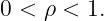



![J [y] ≥ 0 = J [y∗].](https://images.physicslibrary.org/cache/objects/1197/make4ht/AdmissibleFunctionsCalculusOfVariationsFunctionals64x.png)


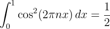
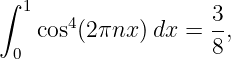
![∫ 1 ∫ 1
J[yn] = 4 π2 cos2(2πnx )dx − 16π4 cos4(2πnx ) dx.
0 0](https://images.physicslibrary.org/cache/objects/1197/make4ht/AdmissibleFunctionsCalculusOfVariationsFunctionals69x.png)
![2 4
J[yn] = 2 π − 6π .](https://images.physicslibrary.org/cache/objects/1197/make4ht/AdmissibleFunctionsCalculusOfVariationsFunctionals72x.png)

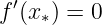
![J [yn ] < J [y∗]](https://images.physicslibrary.org/cache/objects/1197/make4ht/AdmissibleFunctionsCalculusOfVariationsFunctionals74x.png)


![J[y ] < J[y]
∗](https://images.physicslibrary.org/cache/objects/1197/make4ht/AdmissibleFunctionsCalculusOfVariationsFunctionals77x.png)

![∫ 1
J [y] = y(x)2dx.
0](https://images.physicslibrary.org/cache/objects/1197/make4ht/AdmissibleFunctionsCalculusOfVariationsFunctionals80x.png)
![J[yc] = c2.](https://images.physicslibrary.org/cache/objects/1197/make4ht/AdmissibleFunctionsCalculusOfVariationsFunctionals81x.png)
![inf J [y] = 0.
y∈𝒜](https://images.physicslibrary.org/cache/objects/1197/make4ht/AdmissibleFunctionsCalculusOfVariationsFunctionals82x.png)
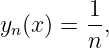
![J[y ] = -1-− → 0.
n n2](https://images.physicslibrary.org/cache/objects/1197/make4ht/AdmissibleFunctionsCalculusOfVariationsFunctionals84x.png)


![Φ (𝜖) = J[y + 𝜖η ].](https://images.physicslibrary.org/cache/objects/1197/make4ht/AdmissibleFunctionsCalculusOfVariationsFunctionals88x.png)
![|
-d- ||
δJ[y;η] = d𝜖J [y + 𝜖η ]| .
𝜖=0](https://images.physicslibrary.org/cache/objects/1197/make4ht/AdmissibleFunctionsCalculusOfVariationsFunctionals89x.png)


