Calculus of Variations: The Fundamental Lemma
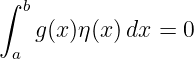
CV02 ended with the identity
for fixed-endpoint variations, after integration by parts. If y is stationary, this integral vanishes for
every admissible variation η.
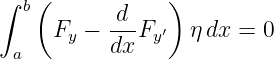
The decisive question is then
If an integral against every sufficiently localized test function is zero, what can
be concluded about the function multiplying that test function?
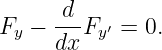
The answer is the Fundamental Lemma of the Calculus of Variations. In its classical form it says
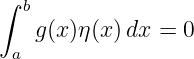
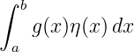
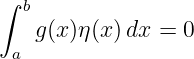
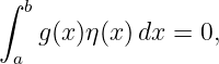
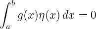
that a continuous function g satisfying
for every admissible test function η must satisfy
throughout the interval.
This theorem is the logical hinge of the Euler–Lagrange derivation. It is not valid because one
can “cancel” η from an integral. It is valid because the family of test functions is rich
enough to probe arbitrarily small regions. If g were positive or negative anywhere, one
could localize a test function near that region and force the integral to have the same
sign.
1 Learning objectives
After this entry, the reader should be able to
- define the support and compact support of a test function;
- explain the localization principle behind variational test functions;
- state the classical Fundamental Lemma with its hypotheses;
- prove the lemma by contradiction using a localized nonnegative bump function;
- identify exactly where continuity of g enters the proof;
- derive the equivalent fixed-endpoint formulation;
- explain why checking only one or finitely many variations is insufficient;
- understand why the conclusion becomes “almost everywhere” for merely integrable
functions;
- apply the lemma to an integral identity arising from a first variation; and
- distinguish an integral identity from the pointwise differential equation that follows
from the lemma.
2 Test functions and support
The proof depends on the ability to choose variations that are concentrated in small parts of the
interval.
2.1 Support
For a function η : (a,b) → ℝ, the support is the closure of the set on which η is nonzero:
A function has compact support in (a,b) if its support is a compact subset of the open interval.
Such a function vanishes not only at the endpoints but in entire neighborhoods of the
endpoints.
The standard notation
denotes infinitely differentiable functions with compact support in (a,b). These are often called test
functions or bump functions.
2.2 Why compact support is useful
Suppose one wants to determine whether an unknown continuous function g is positive near some
point x0. A test function can be chosen so that
- η(x) ≥ 0 everywhere;
- η is not identically zero; and
- η vanishes outside a small interval surrounding x0.
Then the integral
receives contributions only from that small neighborhood. Test functions therefore provide a
mathematical microscope: they allow an integral statement to detect local behavior.
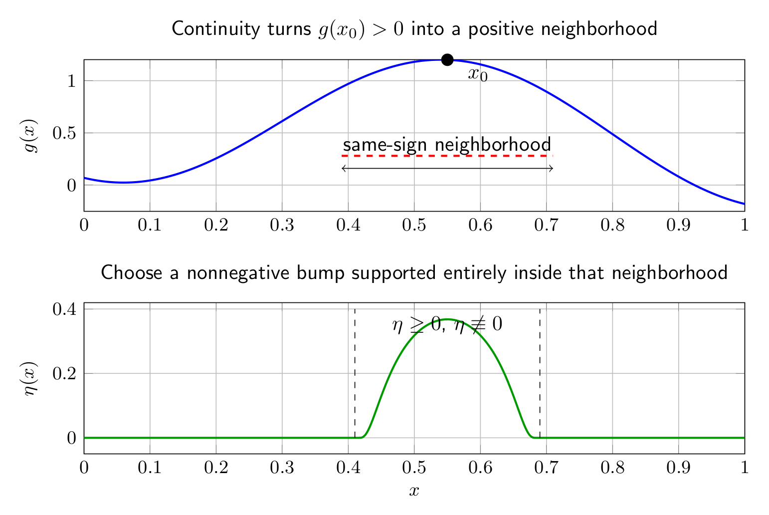
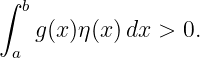
Figure. Localization mechanism behind the Fundamental Lemma. If a continuous g is
positive at x0, then continuity makes it positive on a whole neighborhood of x0. A
nonnegative bump function supported inside that neighborhood forces ∫
gη dx > 0.
3 The classical Fundamental Lemma
Theorem: Fundamental Lemma of the Calculus of Variations. Let
Suppose
for every test function
Then
Because g is continuous on [a,b], the same conclusion extends to the endpoints by continuity, so
g ≡ 0 on [a,b].
4 Proof by localization and contradiction
The proof is short, but each step carries important information.
4.1 Step 1: assume the conclusion is false
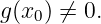
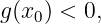
Suppose, for contradiction, that g is not identically zero. Then there is some point x0 ∈ (a,b) such
that
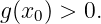
There are two sign cases. It is enough to prove one, because the other is identical after changing
signs. Assume
4.2 Step 2: use continuity
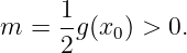
Let
Because g is continuous at x0, there exists r > 0 small enough that
and
for every x ∈ (x0 − r,x0 + r).
This is the exact point at which continuity enters the classical proof. A positive value at one point
is promoted to a positive lower bound on an entire neighborhood.
4.3 Step 3: choose a localized nonnegative test function
Choose
such that
and η is not identically zero.
For example, after rescaling, one may use a standard smooth bump of the form
Its exact formula is not important. What matters is that it is nonnegative, nonzero, smooth, and
supported entirely inside the region where g > m.
4.4 Step 4: determine the sign of the integral
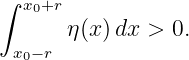
Since η vanishes outside (x0 − r,x0 + r),
On this interval,
and
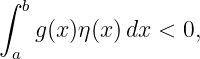
Therefore
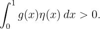
Because m > 0 and η is nonnegative and not identically zero,
Hence
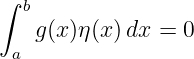
But the hypothesis says that this integral equals zero for every test function. This is a
contradiction.
4.5 Step 5: exclude the negative case
If instead
continuity gives a neighborhood on which g remains strictly negative. The same nonnegative bump
function then yields
again contradicting the hypothesis.
Therefore no point with g(x0)≠0 can exist. Thus
throughout (a,b), and continuity extends the result to [a,b].

Figure. Logical structure of the classical proof. A single nonzero value of a continuous g
creates a same-sign neighborhood. A localized nonnegative test function then makes the
integral nonzero, contradicting the assumption that it vanishes for every test function.
5 Equivalent fixed-endpoint formulation
Many introductory variational derivations use variations satisfying
rather than explicitly introducing compact support.
A useful corollary is therefore the following.
Corollary. Let g ∈ C([a,b]). Suppose
for every continuously differentiable function η satisfying
Then g ≡ 0 on [a,b].
Reason. Every smooth compactly supported test function in (a,b) also satisfies the endpoint
conditions. Thus the hypothesis includes the test functions required by the Fundamental Lemma,
so the theorem applies immediately.
This illustrates a general logical rule: if an integral identity is known for a large class of variations,
it is valid for any smaller test-function class contained within it. One may therefore restrict
attention to especially useful localized variations.
6 Why the test function cannot be cancelled
A common informal statement is
Since η is arbitrary, ∫
gη dx = 0 implies g = 0.
The conclusion is correct under the hypotheses of the lemma, but the language can hide the actual
logic. There is no algebraic cancellation rule
for one fixed η.
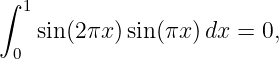
For example, on [0, 1] let
and choose only
Orthogonality gives
although g is certainly not zero.
But if one is also allowed to choose
then
The theorem works because the identity holds for every admissible test function, including
localized functions specifically chosen to expose any nonzero region of g.
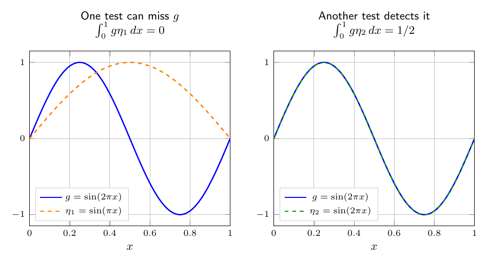
Figure. One test direction can miss a nonzero function through orthogonality. The
Fundamental Lemma requires the integral identity for an entire separating class of test
functions, not for one selected variation.
7 A useful weighted-square test
Sometimes the nonzero character of an integral can be demonstrated without a compactly
supported bump.
Suppose on [0, 1]
Choose the endpoint-zero test function
Then
and
Since x(1 −x) > 0 for 0 < x < 1 and g2 ≥ 0, the integrand is nonnegative and not identically zero.
Therefore
Thus this g cannot satisfy the hypothesis of the Fundamental Lemma.
This argument is useful pedagogically, but it is not a replacement for the localized proof. Its
admissibility depends on the regularity of g, whereas the bump-function proof keeps the test
function independently smooth and makes the localization mechanism explicit.
8 Where continuity matters
The classical statement concluded
That pointwise conclusion uses continuity. If a function is allowed to differ from zero
only on a set of measure zero, ordinary integration cannot detect those exceptional
values.
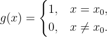
For example, consider the function
For every continuous test function η,
because changing the value of an integrand at one point does not change its Riemann or Lebesgue
integral. Yet g(x0) = 1.
Thus without continuity one should not expect pointwise equality everywhere. The natural modern
conclusion is equality almost everywhere.
9 Modern weak form
The functional-analytic version of the lemma is often stated as follows.
Weak Fundamental Lemma. Let
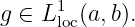
If
for every
then
for almost every x ∈ (a,b).
In the language of distributions, the hypothesis says that the distribution induced by g is the zero
distribution. Two locally integrable functions represent the same distribution exactly when they
agree almost everywhere.
The classical theorem is recovered immediately when g is continuous: if a continuous function is
zero almost everywhere but nonzero at one point, continuity would make it nonzero on an interval
of positive length, a contradiction. Hence continuity upgrades almost-everywhere equality to
pointwise equality.
A full proof of the Lloc1 version belongs to real analysis and distribution theory. The classical
localized-bump proof above contains the physical intuition needed for the variational calculations
in this course.
10 Vector-valued extension
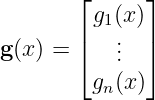
Physics often produces several coupled dependent variables. Suppose
is continuous and
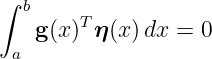
for every smooth compactly supported vector test function η.
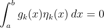
Choose a test function with only its kth component nonzero. The integral reduces to
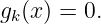
for every scalar test function ηk. The scalar Fundamental Lemma implies
Since this holds for every component,
This componentwise argument is the basis for coupled Euler–Lagrange equations in systems with
many generalized coordinates or fields.
11 Application to the first variation
Return to the first-order functional
CV02 derived
After integration by parts,
For fixed endpoints,
so
If y is stationary, then
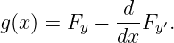
for every admissible variation. Define
Under the regularity assumptions needed to make g continuous, the Fundamental Lemma
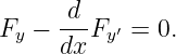
gives
This is the Euler–Lagrange equation.
CV04 will derive this result as a theorem with the regularity assumptions, boundary
conditions, and necessary-condition logic presented in one place. Here the important point is
narrower: the Fundamental Lemma is exactly the mathematical step that turns the integral
statement
into the pointwise statement
12 Necessary condition, not a minimum proof
The Fundamental Lemma does not say that a stationary curve minimizes a functional. It only
allows one to derive a pointwise necessary condition from stationarity.
The logical chain is
The reverse implications do not hold in general. A solution of the Euler–Lagrange equation can be
a maximum, a saddle-type stationary curve, or an extremal that loses minimality after a conjugate
point. Those distinctions require the second variation and the Legendre, Jacobi, and Weierstrass
theories later in the series.
13 Common misconceptions
13.1 Misconception 1: arbitrary means one can divide by η
No. The theorem is not an algebraic division rule. “Arbitrary” means the integral identity holds for
a sufficiently rich family of independent test functions.
13.2 Misconception 2: one nonzero variation is enough to prove g = 0
No. One test function can be orthogonal to a nonzero g. The hypothesis must hold for every test
function in the stated class.
13.3 Misconception 3: a test function must be positive everywhere
No. The proof only needs the ability to choose a nonnegative test function localized inside a region
where g has a definite sign.
13.4 Misconception 4: continuity is merely cosmetic
No. Continuity is what turns a nonzero point value into a same-sign neighborhood and lets the
classical theorem conclude pointwise equality. For locally integrable functions, the correct
conclusion is almost-everywhere equality.
13.5 Misconception 5: the Fundamental Lemma proves a minimum
No. It derives a pointwise stationarity equation. Minimum classification is a separate
problem.
14 Compact theorem map
|
|
| Statement | Conclusion |
|
|
| g ∈ C([a,b]), ∫
gη = 0 for all η ∈ Cc∞ | g = 0 everywhere |
|
|
| same identity for all endpoint-zero C1 variations | g = 0 everywhere |
|
|
| g ∈ Lloc1, ∫ gη = 0 for all C
c∞ tests | g = 0 almost everywhere |
|
|
| identity for one or finitely many selected tests | no such conclusion in general |
|
|
15 What CV04 adds
CV04 will assemble the ingredients developed so far:
- a functional J[y] = ∫
abF(x,y,y′) dx;
- an admissible perturbation y𝜖 = y + 𝜖η;
- the first variation δJ[y; η];
- integration by parts; and
- the Fundamental Lemma.
The result will be a full proof of the Euler–Lagrange necessary condition, including a careful
distinction between stationarity and minimization.
16 Summary
The Fundamental Lemma is a localization theorem. If a continuous function g satisfies
for every smooth compactly supported test function, then g must vanish identically.
The proof is by contradiction. If g were positive or negative at some point, continuity would
preserve that sign on a neighborhood. A nonnegative bump function supported in that
neighborhood would then force the integral to be nonzero.
The family of all test functions is essential: a single test direction can be orthogonal to a nonzero
function. In the modern weak formulation, locally integrable g is determined only up to sets of
measure zero, so the conclusion becomes g = 0 almost everywhere.
For the calculus of variations, the lemma is the bridge from the stationary integral identity
for every admissible variation to the pointwise Euler–Lagrange equation
17 References and further reading
- I. M. Gelfand and S. V. Fomin, Calculus of Variations.
- B. van Brunt, The Calculus of Variations.
- C. Fox, An Introduction to the Calculus of Variations.
- L. C. Evans, Partial Differential Equations, for test functions, weak derivatives, and
distributions.
- R. Courant and D. Hilbert, Methods of Mathematical Physics, for the broader
variational-method viewpoint.

![∫ b ( d )
δJ[y;η] = Fy − --Fy ′ η(x )dx
a dx](https://images.physicslibrary.org/cache/objects/1143/make4ht/CalculusOfVariationsTheFundamentalLemma0x.png)



![g ∈ C ([a,b]).](https://images.physicslibrary.org/cache/objects/1143/make4ht/CalculusOfVariationsTheFundamentalLemma6x.png)



























![∫ b
J[y] = F (x,y,y′)dx.
a](https://images.physicslibrary.org/cache/objects/1143/make4ht/CalculusOfVariationsTheFundamentalLemma53x.png)
![∫ b
′
δJ[y;η] = a (Fy η + Fy′η )dx.](https://images.physicslibrary.org/cache/objects/1143/make4ht/CalculusOfVariationsTheFundamentalLemma54x.png)
![∫ ( )
b b -d-
δJ[y;η] = [Fy ′η]a + Fy − dx Fy′ η dx.
a](https://images.physicslibrary.org/cache/objects/1143/make4ht/CalculusOfVariationsTheFundamentalLemma55x.png)

![∫ b( )
δJ [y;η ] = Fy − d-Fy ′ η dx.
a dx](https://images.physicslibrary.org/cache/objects/1143/make4ht/CalculusOfVariationsTheFundamentalLemma57x.png)
![δJ [y;η] = 0](https://images.physicslibrary.org/cache/objects/1143/make4ht/CalculusOfVariationsTheFundamentalLemma58x.png)


![local extremum =⇒ δJ [y; η] = 0 for all admissible η =⇒ Euler–Lagrange equation.](https://images.physicslibrary.org/cache/objects/1143/make4ht/CalculusOfVariationsTheFundamentalLemma63x.png)