Acoustic Waves, Sound Intensity, and Acoustic Impedance
Sound is a mechanical disturbance that propagates through a material medium.
In a fluid, the simplest acoustic wave is a small longitudinal disturbance of:
- pressure,
- density,
- particle velocity.
The word particle here refers to a small material element of the fluid, not to an isolated
microscopic molecule.
For a uniform fluid at equilibrium pressure
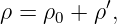
and density
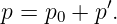
write
and
The acoustic quantities
and
are assumed small compared with the equilibrium values.
If
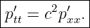
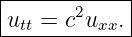
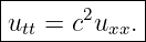
is the longitudinal particle velocity, the linear acoustic equations lead to the wave equation
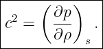
where
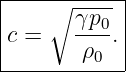
For an ideal gas undergoing small adiabatic disturbances,
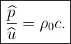
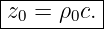
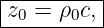
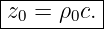
A progressive plane wave has the characteristic specific acoustic impedance
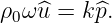
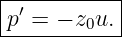
Pressure and particle velocity are then related by
for a wave traveling in the positive
direction.
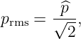
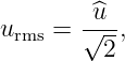
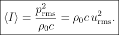
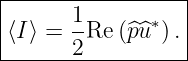
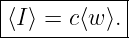
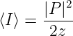
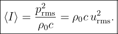
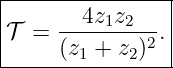
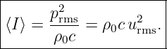
The time-averaged sound intensity of a harmonic plane wave can be written
These relations connect the mechanics of a fluid directly to measurable sound pressure and energy
flow.
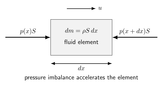
Figure 1. A small fluid element is compressed and accelerated by pressure differences across its
faces. Linear acoustics follows from mass conservation, momentum conservation, and the relation
between pressure and density changes.
1 Equilibrium and acoustic perturbations
Let the undisturbed fluid be at rest:
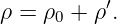
Write the total density and pressure as
and
The acoustic approximation requires
and particle velocities small compared with the sound speed:
Products of two acoustic perturbations are then second order and are neglected in the linear
theory.
2 Mass conservation
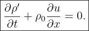
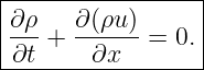
In one dimension, the exact continuity equation is
Insert
Because
is constant,
The product
is second order in the acoustic disturbance.
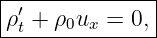
Neglecting it gives the linear continuity equation
A local velocity convergence therefore increases the density perturbation.
3 Momentum conservation
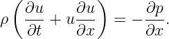
For an inviscid fluid in one dimension, Euler’s equation is
The convective term
is second order.
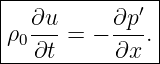
Replacing
by
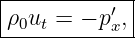
in the first-order term gives
Pressure gradients accelerate the fluid particles.
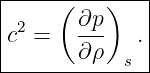
4 Equation of state and sound speed
For sufficiently rapid small-amplitude sound propagation, heat exchange over one acoustic cycle is
often negligible.
The compression is then approximately adiabatic.
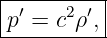
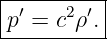
To first order,
where
This Thermodynamic derivative is the square of the sound speed.
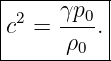
For an ideal gas,
for an adiabatic change.
Differentiating gives
5 Pressure wave equation
Use
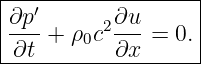
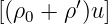
The continuity equation becomes
Differentiate with respect to time:
Differentiate the momentum equation with respect to
Eliminating
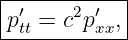
gives
6 Particle-velocity wave equation
Differentiate the momentum equation with respect to time:
Differentiate the pressure form of continuity with respect to
Therefore
Pressure and particle velocity both propagate at the same sound speed.
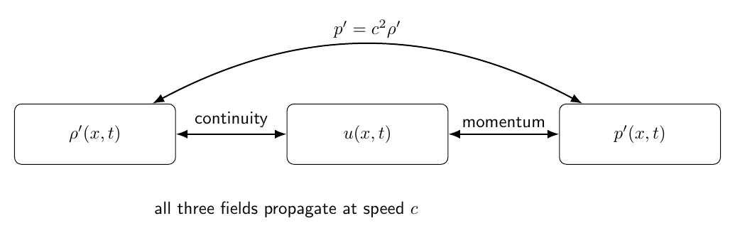
Figure 2. Linear acoustics couples three perturbation fields. Continuity connects density to
particle-velocity gradients, momentum connects particle acceleration to pressure gradients, and
the equation of state connects pressure and density.
7 Sinusoidal plane wave
Consider a positive-direction plane wave
The wave equation requires
Assume
The momentum equation gives
Since
Thus pressure and particle velocity are in phase for a positive-direction progressive plane
wave.
8 Characteristic specific acoustic impedance
Define
Then
for a positive-direction progressive plane wave.
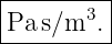
The SI units are
| [z0] | =   | (54)
|
| = Pas∕m. | (55) |
The unit
is also called the rayl.
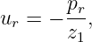
For a negative-direction progressive wave,
The minus sign reflects the reversed direction of the particle-velocity field for a given pressure
phase.
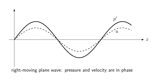
Figure 3. In a progressive plane wave traveling to the right, acoustic pressure and particle velocity
are in phase. Their amplitude ratio is the characteristic specific acoustic impedance z0 = ρ0c.
9 Acoustic intensity
Acoustic intensity is the rate of acoustic energy flow per unit area.
In one dimension the instantaneous intensity is
In three dimensions, the acoustic intensity vector is
Its SI unit is
A positive value of
means net energy flow in the positive
direction.
10 Average intensity of a harmonic plane wave
For a right-moving harmonic plane wave,
and
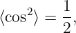
Then
Since
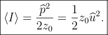
Using
Since
and
11 Complex-amplitude intensity
Let
and
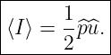
Then the time-averaged intensity is
This form remains useful when pressure and particle velocity are not exactly in phase.
12 Acoustic energy density
The instantaneous acoustic energy density has two contributions.
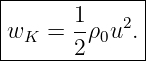
The kinetic contribution is
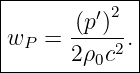
The compressional contribution is
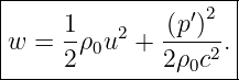
Thus
For a progressive plane wave,
Therefore
instantaneously.
The kinetic and compressional energy densities are equal.
13 Energy density and intensity
For a progressive plane wave,
Using
But
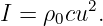
Therefore
for an ideal progressive plane wave.
Likewise,
This is the acoustic analogue of energy density multiplied by transport speed.
14 Example 1: characteristic impedance of air
Take representative room-temperature values
and
Then
| z0 | = ρ0c | (89)
|
| = (1.204)(343) | (90)
|
| ≈ 413 Pas∕m. | (91) |
This is the characteristic specific acoustic impedance of the air for the assumed conditions.
15 Example 2: intensity from sound pressure
Let
in the same air.
Then
| ⟨I⟩ | =  | (93)
|
| ≈ 9.69 × 10⁻⁵ W∕m2. | (94) |
The corresponding particle-velocity RMS amplitude is
| urms | =  | (95)
|
| ≈ 4.84 × 10⁻⁴ m∕s. | (96) |
The material particles move much more slowly than the wave propagates.
16 Spherical spreading
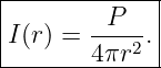
A point-like source radiating acoustic Power
uniformly in all directions distributes that power over a sphere of area
Neglecting absorption,
Therefore
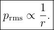
Since
the far-field pressure amplitude scales approximately as
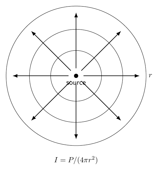
Figure 4. For an ideal point source in a lossless free field, the same acoustic power crosses
increasingly large spherical surfaces. Intensity therefore falls as 1∕r2, while pressure amplitude
falls as 1∕r.
17 Example 3: spherical intensity
Suppose a source radiates
uniformly.
At
| I | =  | (105)
|
| ≈ 1.99 × 10⁻² W∕m2. | (106) |
At
the intensity is one fourth as large:
Doubling distance reduces free-field intensity by a factor of four.
18 Sound intensity level
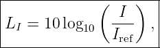
Because audible intensities span many orders of magnitude, a logarithmic scale is useful.
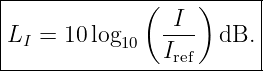
Define the sound intensity level
For sound in air, a conventional reference intensity is
An increase in intensity by a factor of
raises the level by
A factor of
raises it by
19 Sound pressure level
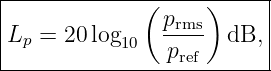
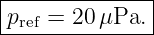
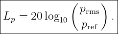
For sound pressure in air, define
with the conventional reference pressure
The factor
rather than
appears because intensity is proportional to pressure squared when the impedance is
fixed:
20 Example 4: pressure level
For
| Lp | = 20 log 10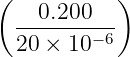 | (121)
|
| = 20 log 10(104) | (122)
|
| = 80.0 dB. | (123) |
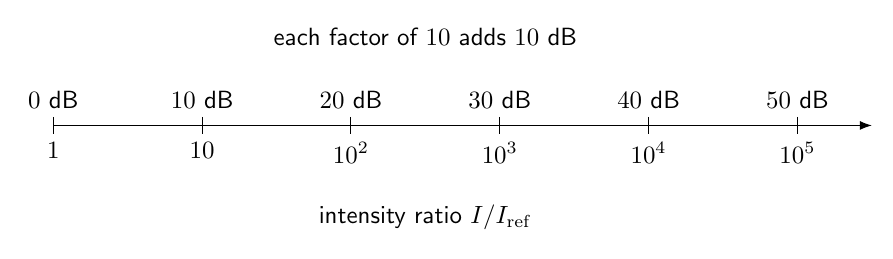
Figure 5. The decibel scale is logarithmic. Multiplying intensity by ten adds 10 dB, while
multiplying pressure amplitude by ten adds 20 dB when the acoustic impedance is unchanged.
21 Distance and level in a free field
For ideal spherical spreading,
If the distance doubles,
Thus
| LI,2 − LI,1 | = 10 log 10 | (126)
|
| ≈−6.02 dB. | (127) |
The familiar approximately
drop per distance doubling is a consequence of ideal spherical spreading, not a universal law for
every acoustic environment.
22 Specific acoustic impedance
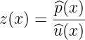
The ratio of complex acoustic pressure to complex particle velocity at a point is the specific
acoustic impedance:
In general,
can be complex and position dependent.
For a positive-direction progressive plane wave in a lossless fluid,
The characteristic value
is real.
23 Acoustic impedance based on volume velocity
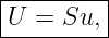
In ducts and acoustic networks, it is often convenient to use the volume velocity
where
is cross-sectional area.
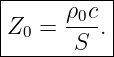
The acoustic impedance is then
For a uniform progressive plane wave in a duct,
Its SI units are
Thus:
- specific acoustic impedance uses particle velocity,
- acoustic impedance uses volume velocity.
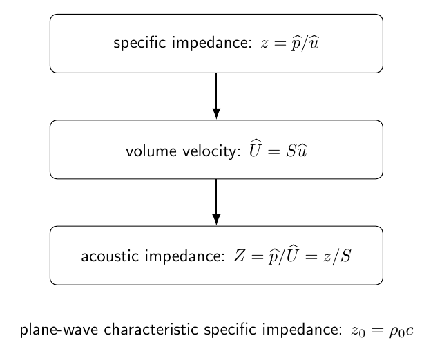
Figure 8. Specific acoustic impedance relates pressure to particle velocity, while acoustic
impedance relates pressure to volume velocity. For a uniform duct, the two differ by the
cross-sectional area.
24 Normal-incidence interface
Consider a plane wave normally incident on a boundary between two lossless fluids.
Let
and
Write the pressure fields as
and
For the corresponding particle velocities,
and
25 Boundary conditions at an ideal fluid interface
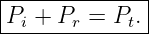
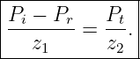
Pressure is continuous:
Normal particle velocity is continuous:
These two conditions determine reflection and transmission.
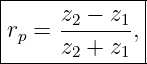
26 Pressure reflection coefficient
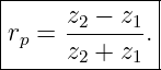
Define
Solving the boundary equations gives
Notice the sign convention compared with the string displacement coefficient in M06-09.
The difference arises because pressure is a force-like variable, while the reflected particle velocity
changes sign with propagation direction.
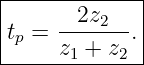
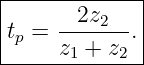
27 Pressure transmission coefficient
Define
Then
The pressure amplitude can exceed the incident pressure amplitude when
This does not imply transmitted power greater than incident power.
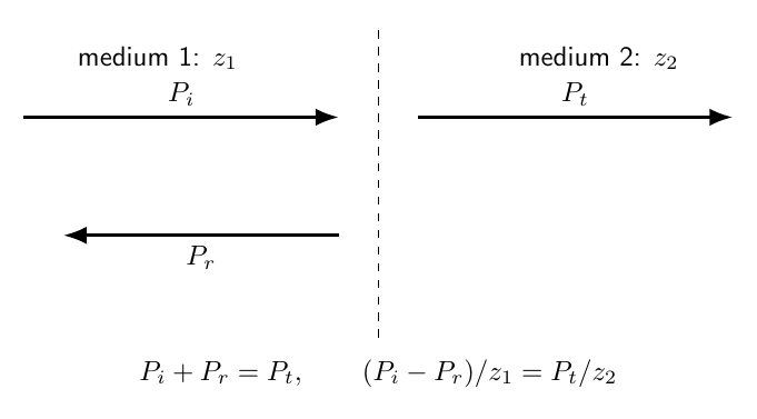
Figure 6. At normal incidence, acoustic pressure and normal particle velocity are continuous
across an ideal fluid interface. Impedance mismatch determines the reflected and transmitted
pressure amplitudes.
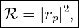
28 Power reflection and transmission
For a plane wave,
when
is the complex peak pressure amplitude and
is real.
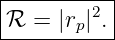
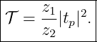
Therefore the reflected power fraction is
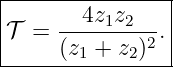
The transmitted power fraction is
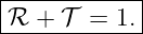
For real positive impedances,
Also,
29 Impedance matching
If
then
There is no reflected plane wave at normal incidence in the ideal model.
Thus, as in the string problem, impedance matching is the reflectionless condition.
30 Example 5: air-to-water impedance mismatch
Use representative values
and
For a plane wave incident from air onto water,
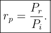
| rp | = 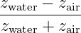 | (164)
|
| ≈ 0.99944. | (165) |
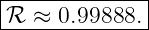
Thus
The transmitted fraction is only
The large impedance mismatch explains why nearly all normally incident acoustic power is
reflected in this idealized calculation.
31 Rigid boundary
A rigid boundary has zero normal particle velocity:
This is the high-impedance limit:
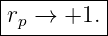
Then
Pressure reflects without inversion.
The reflected particle velocity is inverted.
At the rigid boundary:
- particle velocity has a node,
- acoustic pressure has an antinode.
32 Pressure-release boundary
An ideal pressure-release boundary has
This corresponds to the low-impedance limit:
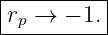
Then
Pressure reflects with inversion.
At the boundary:
- acoustic pressure has a node,
- particle velocity has an antinode.
An open pipe end is often approximated as pressure release in elementary models, although real
open ends require an end correction.
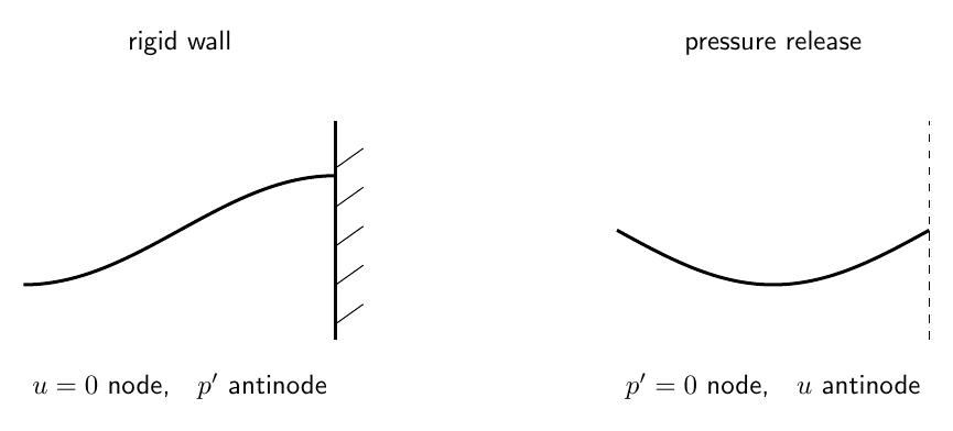
Figure 7. A rigid termination is a particle-velocity node and pressure antinode. An ideal
pressure-release termination is a pressure node and particle-velocity antinode.
33 Standing waves and local impedance
When incident and reflected waves coexist, pressure and particle velocity can acquire different
spatial phases.
The ratio
then depends on position.
It can also become complex.
Therefore
should not be applied blindly to a standing-wave field.
It is the characteristic impedance of a progressive plane wave in the medium.
34 Pressure and velocity nodes
At a rigid wall, a standing wave may be written locally in the form
with the wall at
The associated particle velocity has the form
Thus pressure and particle-velocity nodes are separated spatially by one quarter wavelength.
This geometry is central to acoustic resonators.
35 Coherent and incoherent sound addition
Acoustic intensities cannot always be added by simply adding decibel values.
For mutually incoherent sources, time-averaged intensities add:
The total level is then computed after the intensities are summed.
For coherent sources, acoustic pressures must be added with their relative phases before calculating
intensity.
Interference can produce enhancement or cancellation.
36 Two equal incoherent sources
If two independent sources each produce the same intensity
then
The level increase is
| ΔL | = 10 log 10(2) | (182)
|
| ≈ 3.01 dB. | (183) |
Thus doubling acoustic intensity adds approximately
37 Connection to string impedance
M06-09 defined the characteristic mechanical impedance of a transverse string as
For a plane acoustic wave,
Both express the same general idea:
A wave impedance relates a force-like field to a velocity-like field for a traveling
wave.
For the string, the force-like quantity is transverse force.
For acoustics, it is pressure.
The exact reflection sign depends on which field amplitude is chosen as the reflection
variable.
38 Common mistakes
- Confusing sound speed with fluid-particle speed.
- Treating acoustic pressure p′ as the total thermodynamic pressure p.
- Retaining second-order terms while claiming to use linear acoustics.
- Using an isothermal derivative where the adiabatic sound-speed derivative is required.
- Forgetting that a right-moving plane wave has p′ = ρ0cu.
- Forgetting the minus sign between pressure and particle velocity for a left-moving plane
wave.
- Writing intensity as pressure alone rather than pressure times particle velocity.
- Using peak pressure in an RMS intensity formula without the factor of two.
- Confusing specific acoustic impedance p∕u with acoustic impedance p∕U.
- Forgetting the cross-sectional area when converting from specific acoustic impedance
to duct acoustic impedance.
- Adding decibel values directly instead of adding physical intensities when appropriate.
- Forgetting that pressure-amplitude transmission can exceed one without violating
energy conservation.
- Using the string displacement reflection sign for acoustic pressure without re-deriving
the boundary conditions.
- Calling an open pipe end exactly pressure release without recognizing the
end-correction approximation.
- Applying z0 = ρ0c locally to an arbitrary standing-wave field.
39 Practice exercises
- Linearize the one-dimensional continuity equation.
- Linearize Euler’s equation for an inviscid fluid initially at rest.
- Combine continuity, momentum, and p′ = c2ρ′ to derive the pressure wave equation.
- Derive the particle-velocity wave equation.
- Starting from the momentum equation, derive p∕u = ρ0c for a right-moving plane
wave.
- Derive the average intensity formulas in terms of peak and RMS quantities.
- Derive the acoustic energy density and show that kinetic and compressional
contributions are equal for a progressive plane wave.
- Derive the inverse-square intensity law for an isotropic point source.
- Show why doubling distance reduces free-field level by approximately 6 dB.
- Derive the relation between sound intensity level and sound pressure level for fixed
acoustic impedance.
- Derive the normal-incidence pressure reflection and transmission coefficients at a fluid
interface.
- Derive the power coefficients and verify ℛ + 𝒯 = 1.
- Reproduce the air-to-water numerical example.
- Derive the pressure and particle-velocity behavior at rigid and pressure-release
boundaries.
- Explain why the local impedance of a standing wave need not equal the characteristic
impedance ρ0c.
40 Summary
Linear acoustics begins with
and
These give
and
For a progressive plane wave,
and
for positive-direction propagation.
The average intensity is
Sound levels use logarithmic scales:
and
At a normal-incidence interface,
and
The power coefficients are
and
Acoustic impedance therefore unifies progressive-wave field ratios, interface reflection, power
transmission, and resonant boundary behavior.
References
References
[1] PhysicsLibrary, M06-10, Fourier Analysis, Wave Packets, and Dispersion.
[2] PhysicsLibrary, M06-09, Waves on Strings: Reflection, Transmission, and Mechanical
Impedance.
[3] PhysicsLibrary, M06-08, Continuous Strings, Standing Waves, and Normal Modes.
[4] A. P. French, Vibrations and Waves, W. W. Norton, 1971.
[5] L. E. Kinsler, A. R. Frey, A. B. Coppens, and J. V. Sanders, Fundamentals of
Acoustics, 4th ed., Wiley, 2000.







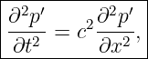






 +

 = 0