Euler’s Equations for Rigid Body Rotation
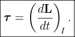
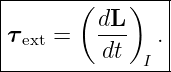
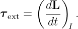
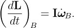
The rotational dynamics law in an inertial frame is
For a general three-dimensional rigid body,
need not be parallel to
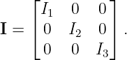
M05-09 introduced
and M05-10 introduced principal axes, in which
The principal axes are fixed in the body, so they rotate relative to an inertial frame.
This creates the key subtlety of three-dimensional rigid body dynamics:
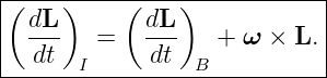
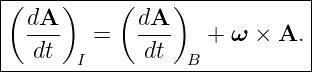
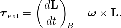
Euler’s equations resolve this by combining angular-momentum dynamics with the derivative rule
for a rotating frame.
The result is
| τ1 = I1ω1 + (I3 − I2)ω2ω3, | | (7)
|
| τ2 = I2ω2 + (I1 − I3)ω3ω1, | | (8)
|
| τ3 = I3ω3 + (I2 − I1)ω1ω2. | | (9) |
These are Euler’s equations for rigid body rotation in principal-axis body coordinates.
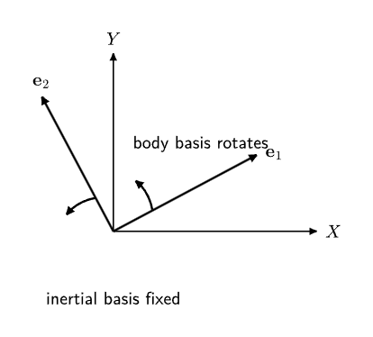
Figure 1. The inertial basis remains fixed while the principal-axis body basis rotates with the
rigid body. Euler’s equations describe angular-momentum dynamics using components resolved in
the rotating body basis.
1 Inertial frame and body frame
Let
be a fixed inertial basis.
Let
be a body-fixed principal-axis basis.
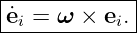
The body basis rotates with angular velocity
relative to the inertial basis.
The angular velocity vector can be written in body components as
The components
can change even while the body basis itself rotates.
2 Derivative of a vector in a rotating frame
For any physical vector
the inertial and rotating-frame derivatives are related by
To see why, write
Differentiate in the inertial frame:
 I I | = Ȧ1e1 + Ȧ2e2 + Ȧ3e3 | (18)
|
| + A1e1 + A2e2 + A3e3. | (19) |
For a basis rotating with angular velocity
Therefore
The remaining component derivatives form
Thus the rotating derivative theorem follows.
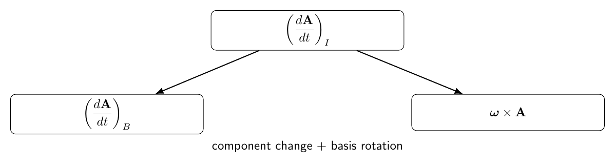
Figure 2. The inertial derivative of a vector contains both the rate of change of its body-frame
components and the change caused by rotation of the body basis itself.
3 Angular momentum in principal-axis coordinates
Choose the body axes to be principal axes through the center of mass.
Then
Therefore
Because the body is rigid,
are constant in the body frame.
4 Derivation of Euler’s vector equation
Start with
Apply the rotating-frame derivative theorem:
In the principal body frame,
and the matrix
is constant.
Thus
Therefore
This is Euler’s equation in compact vector form.
The overdot on the body components means differentiation of the components
with respect to time.
5 Derivation of the component equations
Write
and
The cross product is
| ω × L | = 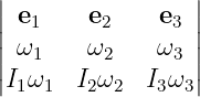 . . | (36) |
Its first component is
The second is
The third is
Therefore
| τ1 = I1ω1 + (I3 − I2)ω2ω3, | | (40)
|
| τ2 = I2ω2 + (I1 − I3)ω3ω1, | | (41)
|
| τ3 = I3ω3 + (I2 − I1)ω1ω2. | | (42) |
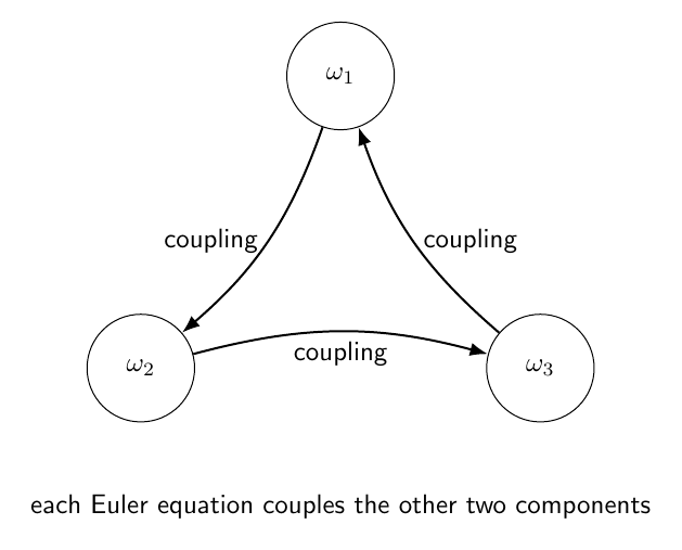
Figure 3. Euler’s equations couple the three body-frame angular-velocity components. Each
equation contains one direct inertial term and one gyroscopic coupling term involving the other
two components.
6 What the coupling terms mean
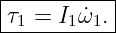
Consider the first equation:
The first term,
resembles the fixed-axis law
The second term,
arises because the principal-axis basis rotates while angular momentum has components along that
rotating basis.
This term is often called a gyroscopic coupling term.
It is not an additional physical torque.
It appears because the angular-momentum components are being differentiated in a rotating body
frame.
7 Why diagonal inertia does not remove dynamic coupling
In principal coordinates the inertia tensor is diagonal:
Nevertheless Euler’s equations remain coupled through products such as
Diagonalization removes algebraic coupling in
It does not remove the kinematic coupling caused by the rotating basis.
This distinction is fundamental.
8 Special case: rotation about one principal axis
Suppose
Then Euler’s equations reduce to
The other two equations become
Thus the familiar scalar law
is recovered for rotation exactly about a principal axis.
9 Example 1: principal-axis spin-up
A rotor has
It initially rotates only about principal axis 3 and experiences torque
Because
Euler’s third equation becomes
Therefore
This is exactly the fixed-axis result.
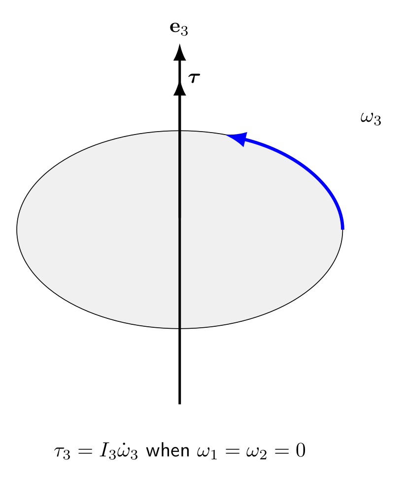
Figure 7. When angular velocity and applied torque lie along the same principal axis and the
other angular-velocity components vanish, Euler’s equations reduce to the scalar law τi = Iiωi.
10 Torque-free Euler equations
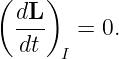
For torque-free motion,
Euler’s equations become
| I1ω1 + (I3 − I2)ω2ω3 = 0, | | (60)
|
| I2ω2 + (I1 − I3)ω3ω1 = 0, | | (61)
|
| I3ω3 + (I2 − I1)ω1ω2 = 0. | | (62) |
Even with zero external torque, the body-frame angular-velocity components can vary.
This does not violate angular-momentum conservation.
The physical vector
is constant in inertial space, while the body axes rotate beneath it.
11 Conservation of angular-momentum magnitude
For torque-free motion,
Therefore
Its magnitude is also constant:
This gives one conserved quadratic surface in angular-velocity component space.
12 Conservation of rotational kinetic energy
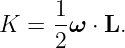
For a rigid body,
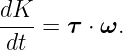
Power delivered by external torque is
Therefore
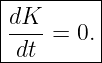
For torque-free motion,
Thus torque-free motion conserves both:
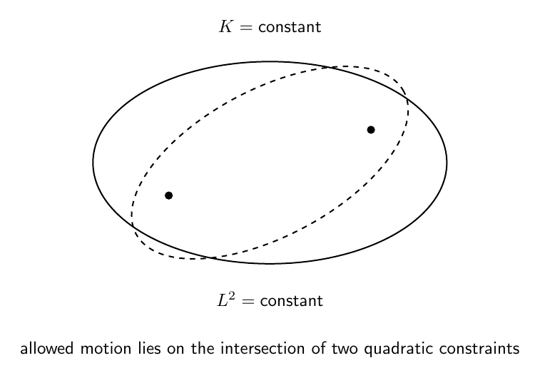
Figure 4. Torque-free motion is constrained simultaneously by constant rotational kinetic energy
and constant angular-momentum magnitude. Their intersection restricts the possible body-frame
angular-velocity components.
13 Checking energy conservation directly from Euler’s equations
Multiply the three torque-free equations by
respectively, and add.
The derivative terms give
The coupling terms sum to
| ![[(I3 − I2) + (I1 − I3) + (I2 − I1)]](https://images.physicslibrary.org/cache/objects/1484/make4ht/EulersEquationsForRigidBodyRotation62x.png) ω1ω2ω3 ω1ω2ω3 | (73)
|
| = 0. | (74) |
Hence
The nonlinear coupling redistributes rotational motion among body components without changing
total kinetic energy.
14 Symmetric rigid body
Consider an axisymmetric body with
For torque-free motion, Euler’s third equation becomes
Therefore
The first two equations become
| I⊥ω1 + (I∥− I⊥)ω2ω3 | = 0, | (79)
|
| I⊥ω2 − (I∥− I⊥)ω3ω1 | = 0. | (80) |
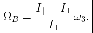
Define
Then
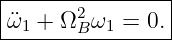
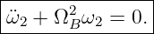
| ω1 | = −ΩBω2, | (82)
|
| ω2 | = ΩBω1. | (83) |
15 Body-frame precession of angular velocity
Differentiate the first symmetric-body equation:
Using
Similarly,
Therefore
The transverse angular-velocity vector rotates around the symmetry axis in the body frame at
angular frequency
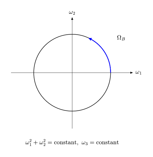
Figure 5. For a torque-free axisymmetric body, ω3 is constant while the transverse components
(ω1,ω2) rotate in the body frame.
16 Example 2: torque-free symmetric body
Let
| I⊥ | = 2.0 kg m2, | (90)
|
| I∥ | = 3.0 kg m2, | (91)
|
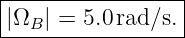
| ω3 | = 10 rad∕s. | (92) |
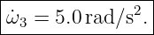
Then
| ΩB | =  (10) (10) | (93)
|
| = 5.0 rad∕s. | (94) |
Thus the transverse body-frame angular-velocity components rotate with frequency
If initially
one convenient solution is
| ω1(t) | = cos(5t), | (97)
|
| ω2(t) | = sin(5t), | (98) |
in radians per second.
17 Steady torque-free rotation about a principal axis
Set two angular-velocity components to zero.
For example,
The torque-free Euler equations then give
Therefore rotation exactly about any principal axis is a torque-free steady solution.
But not every such solution has the same stability.
18 Stability about the minimum principal axis
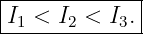
Order the principal moments as
Consider dominant rotation about axis 1:
with small perturbations
To first order, the second and third Euler equations give
| I2ω2 + (I1 − I3)Ωω3 | = 0, | (104)
|
| I3ω3 + (I2 − I1)Ωω2 | = 0. | (105) |
Differentiate the first and substitute the second:
The coefficient is positive.
Therefore the perturbation oscillates rather than grows exponentially.
Rotation about the minimum-moment principal axis is linearly stable.
19 Stability about the maximum principal axis
Now consider dominant rotation about axis 3:
Linearization gives an equation of the form
Again the coefficient is positive.
Thus rotation about the maximum-moment principal axis is also linearly stable.
20 Intermediate-axis instability
Now consider dominant rotation about axis 2:
The linearized first and third equations give
| I1ω1 + (I3 − I2)Ωω3 | = 0, | (110)
|
| I3ω3 + (I2 − I1)Ωω1 | = 0. | (111) |
Differentiate the first equation and substitute the second:
The coefficient multiplying
appears with a minus sign.
Solutions therefore contain exponentially growing and decaying terms.
Rotation about the intermediate principal axis is unstable.
This is the intermediate-axis theorem, also called the tennis-racket theorem.
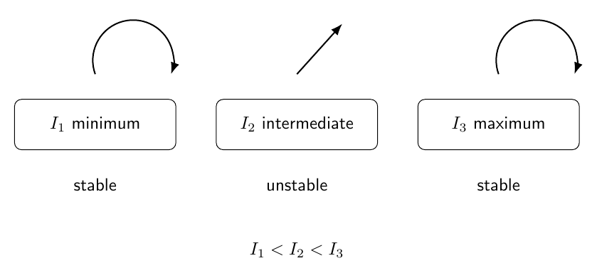
Figure 6. Torque-free rotation about the minimum and maximum principal-moment axes is stable
to small perturbations, while rotation about the intermediate principal-moment axis is unstable.
21 Example 3: growth rate near the intermediate axis
Let
in consistent inertia units.
Suppose the dominant intermediate-axis spin is
The perturbation equation is
where
| λ | = Ω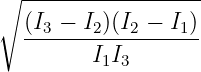 | (117)
|
| = 6 | (118)
|
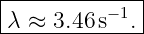
| = 2 s−1. s−1. | (119) |
Thus
Small perturbations can therefore grow rapidly.
22 Applied torque and gyroscopic response
When
Euler’s equations show that an applied torque component does not necessarily change only the
corresponding angular-velocity component.
For example,
Even if
the component
can change if
and
This cross-component response is central to gyroscopes and precession.
23 Example 4: instantaneous coupling
Suppose
| I1 | = 2 kg m2, | (127)
|
| I2 | = 3 kg m2, | (128)
|
| I3 | = 5 kg m2, | (129) |
and at one instant
| ω1 | = 0, | (130)
|
| ω2 | = 4 rad∕s, | (131)
|
| ω3 | = 6 rad∕s. | (132) |
Let
Euler’s first equation gives
| 0 | = 2ω1 + (5 − 3)(4)(6) | (134)
|
| = 2ω1 + 48. | (135) |
Therefore
A body-axis angular-velocity component changes even though no external torque acts along that
body axis.
24 Power in body coordinates
The instantaneous rotational power is
In principal-axis components,
Euler’s equations are consistent with
The gyroscopic coupling terms do not create or destroy energy by themselves.
Their net contribution to
cancels.
25 Angular acceleration versus body-component derivatives
A subtle notation issue deserves emphasis.
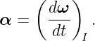
The physical angular acceleration vector is
Using the rotating derivative theorem on
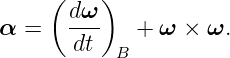
itself gives
But
Therefore
So the body-component derivatives of angular velocity are indeed the body components of angular
acceleration.
This simplification is special to differentiating
itself.
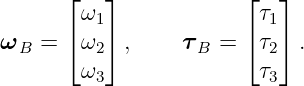
26 Euler equations in matrix form
Let
Then
Therefore
This form is convenient for numerical rigid body simulation.
27 Time integration and attitude
Euler’s equations determine the angular-velocity components.
They do not by themselves determine the body’s orientation.
A complete rigid body simulation must also propagate attitude, for example with:
Thus a three-dimensional simulation contains two coupled pieces:
- rotational dynamics for
- attitude kinematics for the body’s orientation.
This distinction is important in spacecraft, aircraft, robotics, and inertial-navigation
applications.
28 Numerical example: one Euler-equation step
Let
and
Euler’s equations give
| ω1 | = 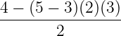 | (154)
|
| = −4 rad∕s2, | (155)
|
| ω2 | = 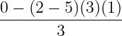 | (156)
|
| = 3 rad∕s2, | (157)
|
| ω3 | = 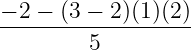 | (158)
|
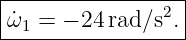
| = −0.8 rad∕s2. | (159) |
Therefore
For a short explicit Euler time step
Thus
A production simulation would normally use a higher-quality integrator and propagate attitude
consistently.
29 Common mistakes
- Writing τ = Iα as the complete law for arbitrary three-dimensional rotation.
- Forgetting that the principal-axis basis rotates with the body.
- Differentiating body components as though the body basis were inertially fixed.
- Omitting the term ω × L.
- Using Euler’s principal-axis component equations in a basis that does not diagonalize
the inertia tensor.
- Mixing inertial-frame components and body-frame components in one equation.
- Treating gyroscopic coupling terms as extra external torques.
- Assuming zero external torque implies constant body-frame angular-velocity
components.
- Assuming torque-free motion means the body rotates about one fixed body axis.
- Forgetting that angular momentum is constant in inertial space during torque-free
motion.
- Forgetting that kinetic energy is also constant for a torque-free rigid body.
- Assuming all three principal-axis rotations have the same stability.
- Forgetting that the intermediate principal axis is unstable.
- Confusing body-frame precession of ω with inertial precession of a symmetry axis.
- Integrating angular velocity without separately propagating attitude.
30 Practice exercises
- Derive the rotating-frame derivative theorem for an arbitrary vector.
- Starting from τ = (dL∕dt)I, derive the compact body-frame equation
- Expand the compact equation into Euler’s three principal-axis component equations.
- Show that rotation exactly about one principal axis reduces Euler’s equations to
τi = Iiωi.
- For torque-free motion, prove directly from Euler’s equations that rotational kinetic energy is
constant.
- Prove that L2 = I
12ω
12 + I
22ω
22 + I
32ω
32 is constant in torque-free motion.
- Derive the torque-free symmetric-body equations for I1 = I2 = I⊥.
- Show that ω12 + ω
22 is constant for the torque-free symmetric body.
- Derive the body-frame precession frequency ΩB = (I∥− I⊥)ω3∕I⊥.
- Linearize the torque-free equations about steady rotation around the minimum principal axis
and show that the perturbations oscillate.
- Repeat for the maximum principal axis.
- Linearize about the intermediate principal axis and show that one perturbation mode grows
exponentially.
- For I1 = 1, I2 = 2, I3 = 3, and Ω = 6 rad/s, reproduce the intermediate-axis growth
rate.
- For I = diag(2, 3, 5) kg m2, ω = (1, 2, 3) rad/s, and τ = (4, 0,−2) N m, compute
ω.
- Explain why Euler’s equations must be combined with attitude kinematics in a full rigid
body simulation.
31 Summary
The inertial angular-momentum law is
For a body-fixed rotating frame,
In principal-axis coordinates,
so
The component equations are
| τ1 = I1ω1 + (I3 − I2)ω2ω3, | | (169)
|
| τ2 = I2ω2 + (I1 − I3)ω3ω1, | | (170)
|
| τ3 = I3ω3 + (I2 − I1)ω1ω2. | | (171) |
For torque-free motion:
- L is constant in inertial space,
- rotational kinetic energy is constant,
- body-frame angular-velocity components can still vary.
For
rotation about the minimum and maximum principal axes is stable to small perturbations, while
rotation about the intermediate principal axis is unstable.
M05-12 uses these results to study gyroscopes, precession, and nutation.
References
References
[1] PhysicsLibrary, M05-10, Principal Axes and Principal Moments of Inertia.
[2] PhysicsLibrary, M05-09, The Inertia Tensor and Products of Inertia.
[3] J. R. Taylor, Classical Mechanics, University Science Books, 2005.
[4] H. Goldstein, C. Poole, and J. Safko, Classical Mechanics, 3rd ed., Addison-Wesley,
2002.
[5] L. D. Landau and E. M. Lifshitz, Mechanics, 3rd ed., Butterworth-Heinemann, 1976.
[6] K. R. Symon, Mechanics, 3rd ed., Addison-Wesley, 1971.

















































































![|--------------------------|
τ-B-=-IB-˙ωB-+--[ωB-×-]IBωB.--](https://images.physicslibrary.org/cache/objects/1484/make4ht/EulersEquationsForRigidBodyRotation114x.png)
![--------------------------------
| − 1 |
ω˙B--=-IB--[τB-−-ωB--×-(IBωB-)].-|](https://images.physicslibrary.org/cache/objects/1484/make4ht/EulersEquationsForRigidBodyRotation115x.png)