Acoustic Resonance in Pipes and Helmholtz Resonators
M06-11 developed acoustic pressure, particle velocity, sound intensity, and acoustic
impedance.
Those ideas now let us understand why pipes, bottles, ducts, and cavities resonate at particular
frequencies.
Two physically different resonance mechanisms will be developed.
The first is a distributed standing-wave resonance in a pipe. Its frequency is determined by how an
acoustic wave fits between boundaries.
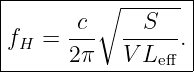
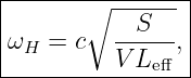
The second is a lumped Helmholtz resonance. A plug of air in a narrow neck acts approximately as
an inertial mass, while compression of the air in the cavity acts approximately as a
spring.
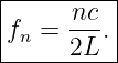
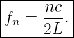
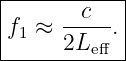
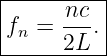
For an ideal uniform pipe, the open-open resonance frequencies are
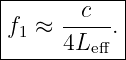
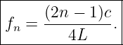
For an ideal pipe closed at one end and open at the other,
A Helmholtz resonator with cavity volume
neck cross-sectional area
and effective neck length
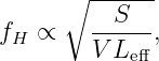
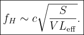
has the approximate resonance frequency
These formulas look simple, but each contains important assumptions and boundary
physics.
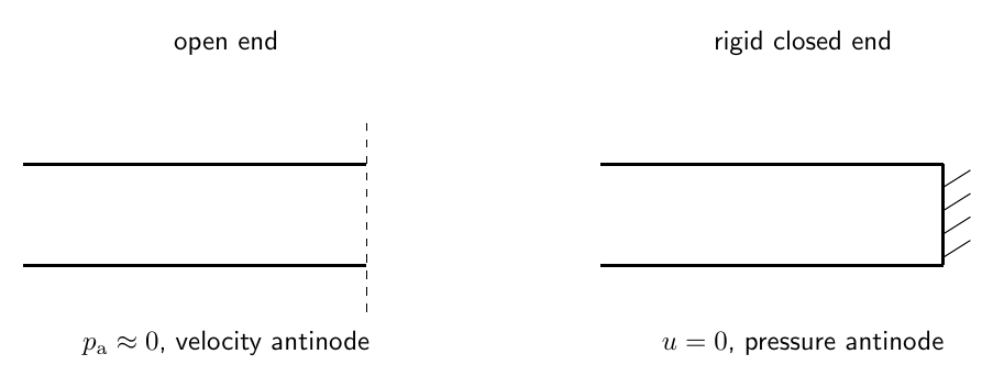
Figure 1. Ideal acoustic boundaries are described by pressure and particle-velocity conditions. An
open end is approximated as a pressure node, while a rigid closed end is a particle-velocity node
and pressure antinode.
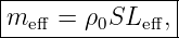
1 Acoustic standing waves in one dimension
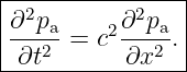
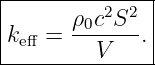
For a uniform lossless duct of constant cross section, the acoustic pressure satisfies
Seek a separated harmonic solution
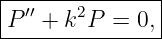
Substitution gives
where
The spatial pressure amplitude therefore has the form
The allowed values of
are selected by the acoustic boundary conditions.
2 Pressure and particle velocity
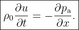
The linearized momentum equation is
For harmonic motion, pressure and particle velocity are spatially shifted relative to one
another.
Where pressure has a standing-wave antinode, particle velocity has a node.
Where pressure has a standing-wave node, particle velocity has an antinode.
This quarter-wavelength spatial offset is the central geometry of pipe resonances.
3 Ideal closed end
At a rigid end, the fluid cannot move Normal to the wall.
Therefore
From the momentum relation, this corresponds to a pressure extremum.
Thus a rigid closed end is:
- a particle-velocity node,
- an acoustic-pressure antinode.
For the spatial pressure function, the ideal boundary condition can be written
4 Ideal open end
An open pipe end communicates with a much larger external region.
In the simplest approximation, the acoustic pressure perturbation at the opening is
small:
Thus an ideal open end is:
- an acoustic-pressure node,
- a particle-velocity antinode.
This ideal condition is not exact at the physical pipe edge.
The effective pressure node lies slightly outside the pipe, producing the end correction developed
later.
5 Open-open pipe
Let a pipe of length
be open at both ends.
Choose
and
at the ideal pressure nodes.
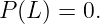
The first boundary condition is
Since
this gives
Therefore
The second boundary condition is
Hence
Therefore
Since
The open-open pipe supports all positive integer harmonics of the fundamental.
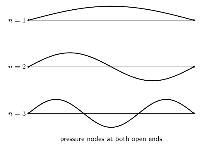
Figure 2. The first three ideal pressure modes of an open-open pipe. Both ends are pressure
nodes. The allowed wavelengths satisfy L = nλn∕2.
6 Open-open fundamental
For
Thus
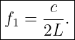
The fundamental frequency is
The pressure has:
- nodes at both ends,
- an antinode at the midpoint.
Particle velocity has the complementary pattern:
- antinodes at both ends,
- a node at the midpoint.
7 Closed-closed pipe
A pipe rigidly closed at both ends has
Using
the condition at
gives
Therefore
The condition at
requires
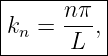
Thus the nonzero acoustic modes have
and
The nonzero resonance frequencies therefore match those of the ideal open-open pipe, although the
pressure and particle-velocity node patterns are interchanged.
8 Closed-open pipe
Now close the left end and open the right end.
At
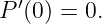
the rigid boundary requires
Therefore
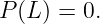
At the open end,
Thus
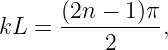
Therefore
so
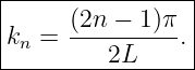
The resonance frequencies are
Only odd multiples of the fundamental appear in this ideal one-dimensional model.
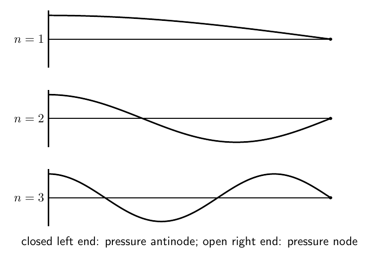
Figure 3. The first three ideal pressure modes of a closed-open pipe. The rigid end is a pressure
antinode and the open end is a pressure node, so only odd multiples of the fundamental occur.
9 Quarter-wave fundamental
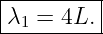
For the closed-open fundamental,
Therefore
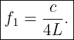
The corresponding fundamental is
This is why a closed-open pipe is called a quarter-wave resonator.
An open-open pipe is a half-wave resonator because
10 Pressure nodes and velocity nodes
Pressure and particle velocity do not have nodes at the same places.
For an ideal standing wave in a uniform duct:
- a pressure node coincides with a particle-velocity antinode,
- a pressure antinode coincides with a particle-velocity node.
The spatial separation between a neighboring pressure node and pressure antinode is
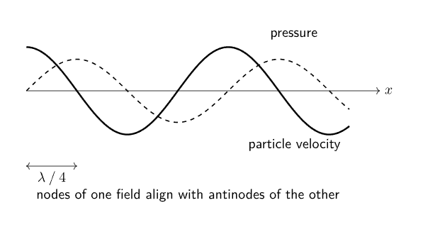
Figure 4. Pressure and particle-velocity Standing Waves are shifted by one quarter wavelength. A
pressure node occurs where particle velocity has an antinode, and vice versa.
11 Example 1: open-open pipe
Take
and
The ideal fundamental is
| f1 | =  | (57)
|
| ≈ 228.7 Hz. | (58) |
The next two resonances are
and
12 Example 2: closed-open pipe
For the same physical length,
| f1 | =  | (61)
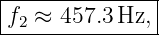
|
| ≈ 114.3 Hz. | (62) |
The next ideal resonances are
and
13 Why the open-end condition is not exact
At a real open end, oscillating air just outside the physical pipe also participates in the
motion.
The acoustic field therefore does not terminate abruptly at the geometric edge.
Instead, the effective pressure node lies a short distance outside the pipe.
This makes the acoustic resonator behave as though it were slightly longer than its measured
geometric length.
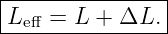
Define
Here
is the open-end correction.
14 Approximate end corrections
The exact end correction depends on geometry.
For a circular pipe of radius
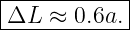
a commonly used low-frequency approximation for one unflanged open end is
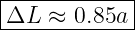
For an idealized flanged circular opening, a larger value near
is often used.
These are approximations, not universal constants.
The correction depends on flange geometry, wall thickness, frequency, and nearby boundaries.
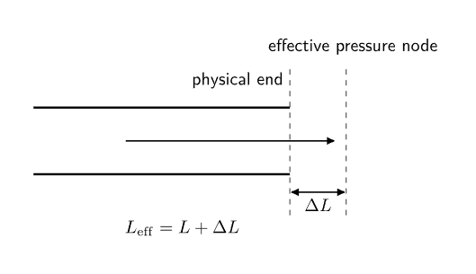
Figure 5. A real open end behaves as though the pressure node were slightly outside the physical
pipe. The effective acoustic length is therefore larger than the geometric length.
15 Open-open pipe with end correction
If both ends are approximately identical and unflanged,
The corrected fundamental is approximately
Since
the corrected resonance frequency is lower than the ideal geometric-length prediction.
16 Closed-open pipe with end correction
If only the open end requires a correction,
Then
17 Example 3: effect of end correction
Consider an open-open circular pipe with
and radius
Use the unflanged estimate
Then
With two open ends,
The corrected fundamental is
| f1 | ≈ | (80)
|
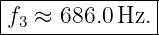
| ≈ 223.3 Hz. | (81) |
The end correction lowers the prediction by about
for this example.
18 Driven acoustic resonance
A pipe resonance is observable when the acoustic system is driven near one of its natural
frequencies.
As in M06-03, damping prevents unbounded growth and produces a finite resonance
peak.
A simple single-mode approximation has the same mathematical form as a driven damped
oscillator:
where
is now a modal coordinate.
Near an isolated acoustic resonance, the response is therefore approximately oscillator-like.
19 Quality factor
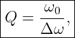
For a weakly damped isolated resonance, define
where
is the full width between the half-power frequencies.
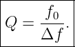
Equivalently,
Large
means:
- a narrow resonance,
- relatively slow energy loss,
- longer ring-down time.
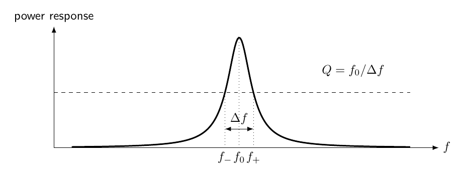
Figure 6. A damped acoustic mode has a finite resonance width. In the weak-damping limit, the
quality factor is approximately Q = f0∕Δf, where Δf is the half-power bandwidth.
20 From distributed pipe resonance to lumped resonance
A long pipe resonance requires a spatial standing-wave pattern.
A Helmholtz resonator is different.
If the cavity dimensions are small compared with the acoustic wavelength, the pressure inside the
cavity is approximately uniform at any instant.
The resonator can then be approximated by:
- an oscillating plug of air in the neck,
- a nearly uniform compressible air volume in the cavity.
This is a lumped-element approximation.
21 Helmholtz resonator geometry
Let:
- V be the cavity volume,
- S be the neck cross-sectional area,
- Leff be the effective neck length,
- ρ0 be the equilibrium air density.
Let
be the displacement of the neck air plug.
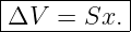
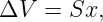
The volume displaced into the cavity is approximately
22 Effective mass of the neck air
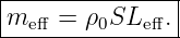
The mass of the moving neck plug is approximated by
The use of
rather than the geometric neck length accounts approximately for fluid outside the neck that
participates in the oscillation.
23 Cavity pressure as a spring
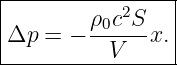
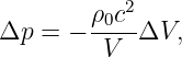
The cavity air is compressed by the volume change.
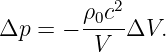
For a small adiabatic compression,
Since
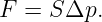
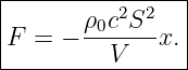
The pressure force on the neck plug is
Therefore
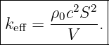
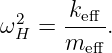
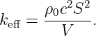
The effective acoustic spring constant is
24 Helmholtz resonance frequency
Newton’s second law for the neck plug is
Thus
Substitute
and
Then
| ωH2 | =  | (103)
|
| =  . | (104) |
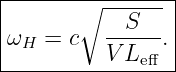
Therefore
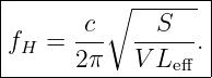
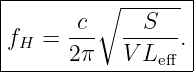
The ordinary frequency is
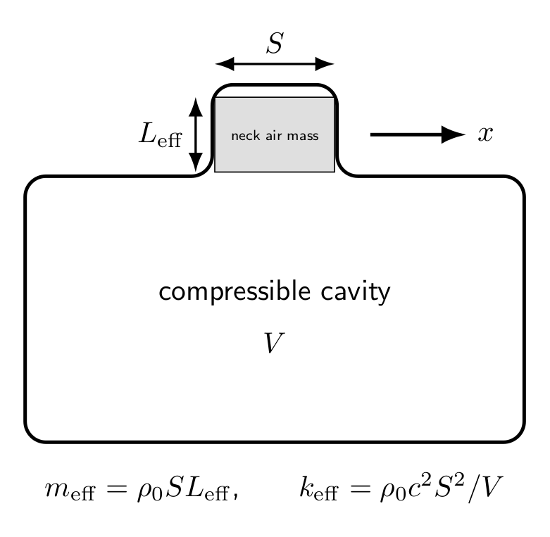
Figure 7. In the Helmholtz approximation, the air in the neck behaves as an inertial mass while
compression of the cavity air provides the restoring spring.
25 Acoustic compliance
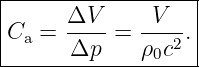
The cavity can also be described through its acoustic compliance.
Define volume displacement
From
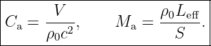
the magnitude of the compliance is
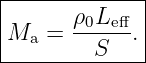
The neck provides acoustic inertance
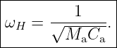
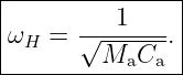
Then
This is exactly the mathematical structure of a mass-spring oscillator.
26 Example 4: bottle-like Helmholtz resonator
Take
which is
Let the neck radius be
so
Take
and
Then
| fH | =  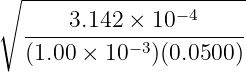 | (118)
|
| ≈ 136.8 Hz. | (119) |
27 How geometry changes Helmholtz frequency
From
we can read off the trends.
Increasing neck area:
Increasing cavity volume:
Increasing effective neck length:
These trends have direct physical interpretations:
- larger neck area strengthens the pressure restoring force relative to neck inertia,
- larger cavity volume makes the cavity more compliant,
- a longer neck increases the moving air mass.
28 Neck end correction
The effective neck length is longer than the geometric neck length because some air just outside
the neck participates in the motion.
Write
The exact correction depends on:
- whether each end is flanged or unflanged,
- neck radius,
- wall thickness,
- cavity geometry,
- frequency.
For introductory calculations, the correction is often represented by a geometry-dependent multiple
of the neck radius.
It should not be treated as a universal single number.
29 Helmholtz resonance versus pipe resonance
The distinction is important.
A pipe resonance is a distributed standing-wave phenomenon.
Its frequency scales primarily as
A Helmholtz resonance is a lumped inertance-compliance oscillation.
Its frequency scales as
A cavity can possess both a low-frequency Helmholtz resonance and higher-frequency distributed
acoustic modes.
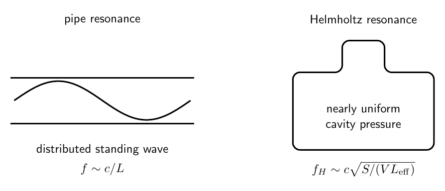
Figure 8. A pipe resonance depends on a spatial standing-wave pattern, while a Helmholtz
resonance treats the cavity pressure as nearly uniform and the neck air as a lumped oscillating
mass.
30 Validity of the Helmholtz approximation
The lumped Helmholtz model requires the cavity to be acoustically compact.
A useful condition is that the cavity’s characteristic dimensions be small compared with the
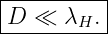
acoustic wavelength:
Then pressure can be approximated as nearly uniform throughout the cavity.
If the frequency becomes high enough that significant spatial pressure variation develops inside the
cavity, distributed cavity modes must be included.
31 Losses and resonance width
Real acoustic resonators lose energy through:
- viscous boundary layers,
- thermal conduction,
- radiation from openings,
- turbulence,
- material losses,
- leakage.
These effects broaden the resonance and reduce its peak amplitude.
A practical Helmholtz resonator is therefore better modeled as a damped oscillator:
The same resonance concepts developed in M06-03 apply.
32 Example 5: bandwidth and quality factor
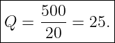
Suppose an acoustic resonance has
and measured half-power frequencies
Then
Thus
33 Connection to acoustic impedance
At resonance, the reactive parts of an acoustic system can cancel.
In a lumped Helmholtz model:
- neck inertance contributes an inertia-like reactance,
- cavity compliance contributes a spring-like reactance.
At
their magnitudes balance.
This impedance viewpoint is the acoustic analogue of resonance in mechanical and electrical
oscillators.
34 Common mistakes
- Calling an open end a particle-velocity node rather than a pressure node.
- Calling a rigid closed end a pressure node rather than a pressure antinode.
- Forgetting that pressure and particle-velocity nodes are interchanged.
- Using the open-open spectrum for a closed-open pipe.
- Forgetting that a closed-open pipe supports odd harmonics in the ideal model.
- Writing the quarter-wave fundamental as c∕(2L) instead of c∕(4L).
- Treating the physical pipe length as exactly equal to the acoustic length.
- Applying a fixed numerical end correction without specifying geometry.
- Adding only one open-end correction to an open-open pipe with two similar ends.
- Confusing a Helmholtz resonance with a quarter-wave pipe resonance.
- Omitting the effective neck length from the Helmholtz formula.
- Treating the cavity pressure as uniform when the cavity dimensions are not small
compared with wavelength.
- Forgetting that resonance peaks have finite width in real systems.
- Confusing the half-power bandwidth with half the bandwidth.
- Using a high-frequency distributed cavity mode formula when the intended model is a
lumped Helmholtz resonator.
35 Practice exercises
- Starting from P′′ + k2P = 0, derive the open-open pipe spectrum.
- Derive the nonzero closed-closed pipe spectrum.
- Derive the closed-open pipe spectrum.
- Draw the pressure and particle-velocity node patterns for the first three open-open
modes.
- Draw the pressure and particle-velocity patterns for the first three closed-open modes.
- Reproduce Examples 1 and 2 numerically.
- Apply a 0.6a end correction to a specified circular open pipe and compare the corrected
and uncorrected fundamentals.
- Explain physically why end correction lowers resonance frequency.
- Starting from a neck air plug of mass ρ0SLeff, derive the Helmholtz frequency.
- Derive the acoustic compliance Ca = V∕(ρ0c2).
- Derive the acoustic inertance Ma = ρ0Leff∕S.
- Show that ωH = 1∕
 .
- Reproduce the bottle-like Helmholtz numerical example.
- Determine how fH changes if cavity volume is quadrupled while all other parameters
remain fixed.
- Given f0 and half-power frequencies, compute Q.
36 Summary
For a uniform ideal open-open pipe,
For a uniform ideal closed-open pipe,
An open end is approximately:
- a pressure node,
- a particle-velocity antinode.
A rigid closed end is:
- a pressure antinode,
- a particle-velocity node.
Real open ends require an effective length
For a Helmholtz resonator,
and
Therefore
and
The acoustic-compliance form is
Thus
Pipe resonance and Helmholtz resonance are therefore two different realizations of the same
broader idea: energy repeatedly exchanges between inertial and restoring mechanisms while
boundary conditions select the allowed motion.
References
References
[1] PhysicsLibrary, M06-11, Acoustic Waves, Sound Intensity, and Acoustic Impedance.
[2] PhysicsLibrary, M06-03, Driven Harmonic Motion and Resonance.
[3] PhysicsLibrary, M06-08, Continuous Strings, Standing Waves, and Normal Modes.
[4] A. P. French, Vibrations and Waves, W. W. Norton, 1971.
[5] L. E. Kinsler, A. R. Frey, A. B. Coppens, and J. V. Sanders, Fundamentals of
Acoustics, 4th ed., Wiley, 2000.