Driven Harmonic Motion and Resonance
A free oscillator evolves from its initial state.
A driven oscillator also receives energy from an external time-dependent force.
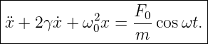
The standard linear model is
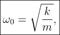
Here:
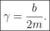
Define
and
Then
The solution contains two physically distinct parts:
The transient
depends on initial conditions and decays when
The steady-state response
is determined by the driving force and remains after the transient has disappeared.
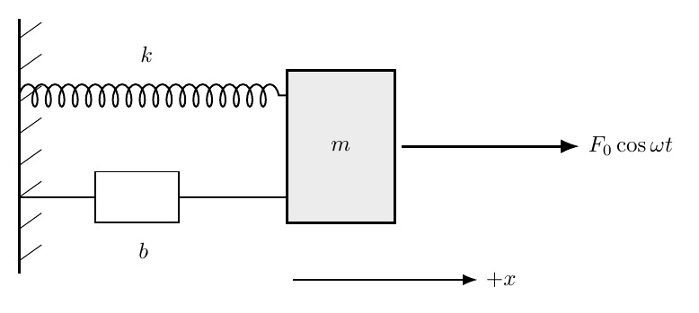
Figure 1. A driven damped oscillator contains an elastic restoring force, a viscous damping force,
and an externally applied periodic force F0 cosωt.
1 Homogeneous and particular solutions
The differential equation is linear:
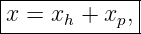
Its general solution is
where
and
The homogeneous solution is exactly the damped free motion developed in M06-02.
For an underdamped system,
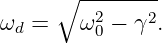
with
Because this part decays, the long-time response is governed by the particular solution.
2 Why the steady state oscillates at the driving frequency
The external force is sinusoidal at angular frequency
For a linear time-invariant oscillator, a sinusoidal input produces a sinusoidal steady-state response
at the same frequency.
The amplitude and phase can change, but the steady-state frequency is the driving
frequency.
Write
The response amplitude
and phase lag
depend on
3 Direct sine-cosine derivation
Assume
Then
and
Substitute into
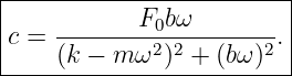
The cosine coefficient gives
The sine coefficient gives
Solving,
and
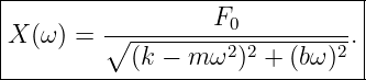
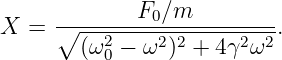
4 Steady-state amplitude
Because
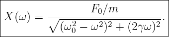
Dividing numerator and denominator by
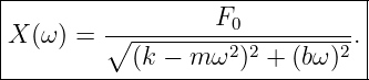
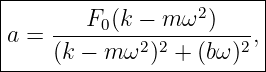
This is the frequency-response amplitude of the driven oscillator.
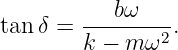
5 Steady-state phase lag
From
The quadrant-aware form is
Equivalently,
The displacement lags the driving force by
6 Complex-exponential derivation
The same result follows more compactly with complex notation.
Represent the force as the real part of
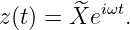
Seek
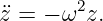
Then
and
Substitution gives
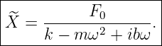
Therefore
The physical response is
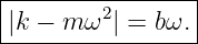
The magnitude of
is
and its argument is
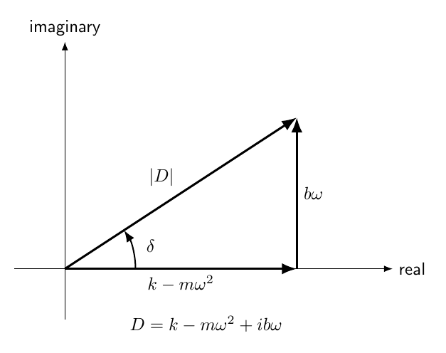
Figure 3. In the complex response denominator, k − mω2 is the in-phase stiffness-inertia term and
bω is the quadrature damping term. Their vector magnitude determines the inverse response
amplitude.
7 Transient plus steady state
For an underdamped oscillator,
The constants
and
are determined by the initial state.
At long times,
Thus
The system loses memory of its initial state but not of the continuing drive.
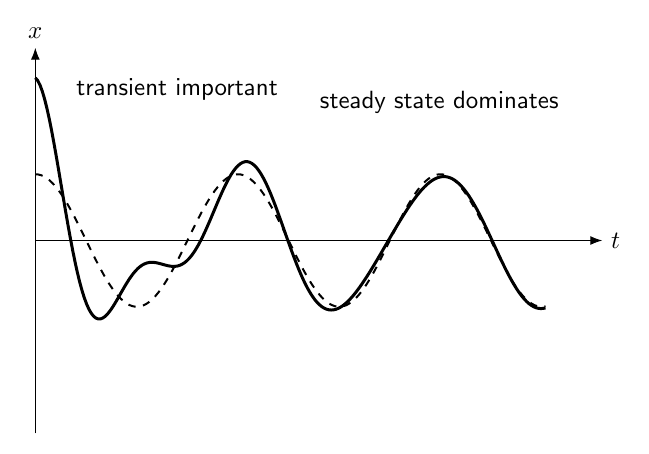
Figure 2. The total response is the sum of a decaying transient and a persistent steady-state
oscillation at the driving frequency.
8 Normalized frequency response
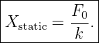
Define the static displacement under force
as
Define
and the damping ratio
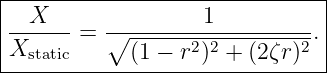
Then
This dimensionless form shows how the response depends only on frequency ratio and damping
ratio.
9 Low-frequency limit
If
then
and
Therefore
Also,
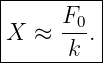
The oscillator follows the slowly changing force almost quasistatically.
10 High-frequency limit
If
the inertial term dominates:
Thus
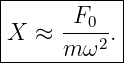
The displacement becomes small, and
The displacement is nearly opposite the applied force.
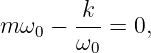
11 At the undamped natural frequency
Set
Then
Therefore
The phase lag is
At
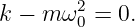
the spring and inertial response terms cancel in the steady-state force balance, leaving damping to
balance the applied force.
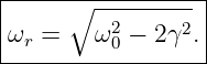
12 Displacement-amplitude resonance
The displacement amplitude is
To maximize
minimize the squared denominator:
Differentiate:
 | = −4ω(ω02 − ω2) + 8γ2ω | (74)
|
| = 4ω![[ω2 − ω2 + 2γ2]
0](https://images.physicslibrary.org/cache/objects/1492/make4ht/DrivenHarmonicMotionAndResonance74x.png) . . | (75) |
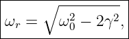
For a nonzero resonance frequency,
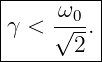
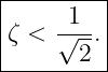
A nonzero displacement-amplitude peak exists only if
Equivalently,
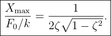
13 Maximum displacement response
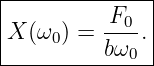
At
The normalized maximum displacement is
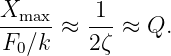
For very light damping,
and
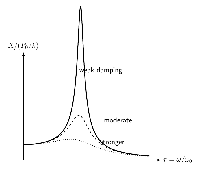
Figure 4. The normalized displacement response develops a tall narrow resonance peak for weak
damping. Increased damping lowers and broadens the peak, and sufficiently strong damping
removes the nonzero-frequency displacement maximum.
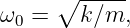
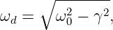
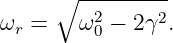
14 Natural frequency is not always the displacement-resonance frequency
Three frequencies should be distinguished:
- undamped natural frequency:
- damped free-oscillation frequency:
- driven displacement-resonance frequency:
For weak damping they are close, but they are not identical.
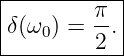
15 Phase response
The phase lag is
Therefore:
- δ → 0 as ω → 0,
- δ = π∕2 at ω = ω0,
- δ → π as ω →∞.
The transition is sharper for weak damping.
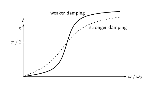
Figure 5. The displacement response changes from nearly in phase with the force at low frequency
to nearly opposite the force at high frequency, passing through a 90∘ lag at ω0.
16 Velocity response
The steady-state velocity is
Its amplitude is
At
The velocity-amplitude response is maximized at
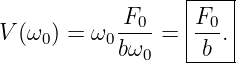
Thus velocity resonance occurs exactly at the undamped natural frequency for viscous
damping.
17 Average power delivered by the drive
The applied force is
The velocity is
The instantaneous input power is
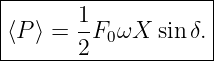
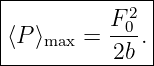
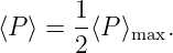
Averaging over one cycle gives
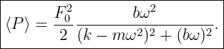
Using the amplitude and phase formulas,
Equivalently,
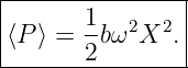
In steady state, average input power equals average power dissipated by damping.
18 Power resonance
The average power is maximized at
At this frequency,
This is another reason to distinguish power resonance from displacement-amplitude
resonance.
For finite damping:
while the maximum average power occurs at
19 Half-power frequencies
Define
and
by
For viscous damping, the condition becomes
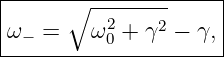
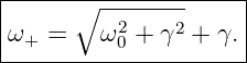
The positive roots are
and
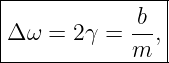
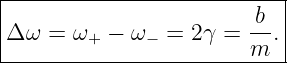
Their difference is exactly
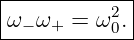
Their product is
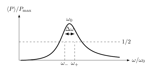
Figure 6. The average absorbed power peaks at ω0. The two half-power frequencies define the
bandwidth Δω = ω+ − ω− = 2γ.
20 Quality factor from resonance bandwidth
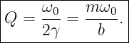
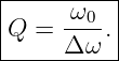
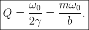
Define
Since
Using
For a lightly damped resonator, large
means:
- a tall displacement-response peak,
- a narrow power-resonance bandwidth,
- slow decay of free oscillations.
21 Example 1: steady-state amplitude and phase
Let
| m | = 1.0 kg, | (118)
|
| k | = 100 N∕m, | (119)
|
| b | = 2.0 kg∕s, | (120)
|
| F0 | = 10 N, | (121)
|
| ω | = 8.0 rad∕s. | (122) |
Then
The in-phase denominator term is
The damping term is
Thus
| X | = 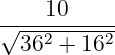 | (126)
|
| ≈ 0.254 m. | (127) |
The phase lag is
| δ | = atan2(16, 36) | (128)
|
| ≈ 0.418 rad | (129)
|
| ≈ 23.96∘. | (130) |
22 Example 2: resonance frequency and quality factor
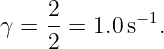
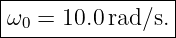
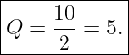
Use the same
Then
The displacement-resonance frequency is
| ωr | = 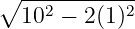 | (133)
|
| =  | (134)
|
| ≈ 9.90 rad∕s. | (135) |
The power-resonance frequency is
The bandwidth is
Therefore
23 Mechanical impedance
The complex displacement relation is
The complex velocity amplitude is
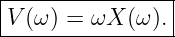
Define mechanical impedance by
Then
| Z | = 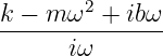 | (142)
|
| = b + i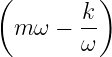 . . | (143) |
The real part
represents dissipation.
The imaginary part represents reactive storage by mass and spring.
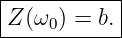
At
so
The impedance is purely resistive at power resonance.
24 Undamped driven oscillator
Set
Then
For
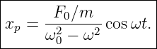
a particular solution is
The denominator becomes small when the drive approaches the natural frequency.
Without damping, however, the behavior at exact resonance must be treated separately.
25 Beating for an undamped oscillator released from rest
Suppose
and
The exact solution is
Use
Then
When
is close to
the rapid oscillation is modulated by a slow envelope.
This is beating.
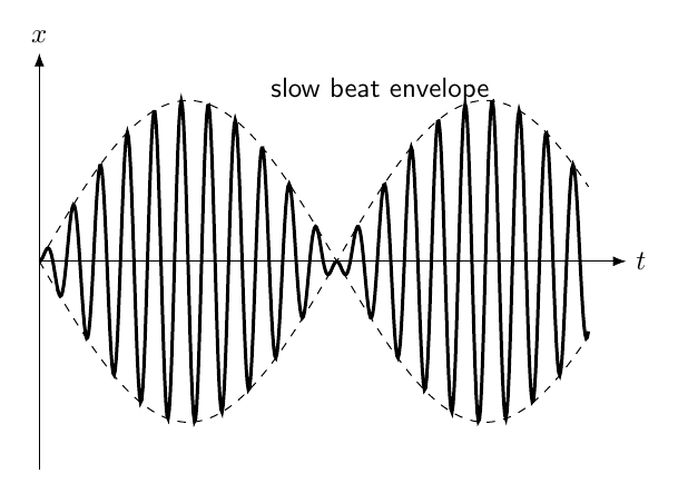
Figure 7. In the undamped oscillator driven near but not exactly at its natural frequency,
interference between the drive-frequency and natural-frequency terms produces beats.
26 Exact undamped resonance
Now set
The ordinary cosine trial particular solution fails because
is already a homogeneous solution.
Try
Substitution gives
Therefore
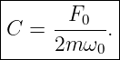
Hence
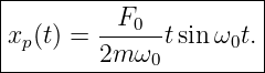
The oscillation amplitude grows linearly with time.
The ideal undamped resonance is therefore not a finite sinusoid of infinite amplitude.
It is a secularly growing response.
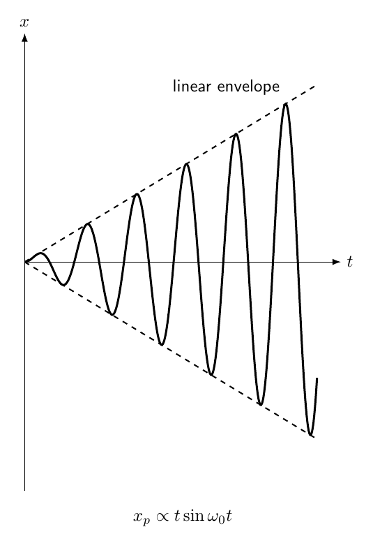
Figure 8. At exact resonance with zero damping, the response contains a factor of t. The envelope
grows linearly rather than approaching a finite steady-state amplitude.
27 Why damping regularizes resonance
With
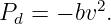
energy is continuously removed at rate
In steady state, the drive supplies exactly the average energy dissipated each cycle.
This balance produces a finite resonance response.
Smaller
means less dissipation per cycle and therefore a larger resonant response.
In the formal limit
the finite damped steady-state picture breaks down at exact resonance and the secular undamped
solution must be used.
28 Resonance as energy transfer
Resonance is fundamentally efficient energy transfer from a periodic drive into an oscillator.
At low frequency, displacement follows the force nearly in phase and velocity is small.
At high frequency, inertia suppresses displacement.
Near
the force is nearly in phase with velocity, so the drive performs positive net work over each cycle
most effectively.
At exact power resonance,
so velocity is in phase with force.
That is why average absorbed power is maximized at
29 Resonance is not always desirable
Resonance can be useful in:
- frequency selection,
- musical instruments,
- sensors,
- resonant cavities,
- mechanical and electrical filters.
It can be dangerous in:
- machinery,
- structures,
- vehicles,
- rotating equipment,
- components subjected to periodic forcing.
The linear oscillator provides the first model for both resonance enhancement and resonance
avoidance.
30 Common mistakes
- Assuming the steady-state response oscillates at the natural frequency rather than the
driving frequency.
- Forgetting that the total solution contains both transient and steady-state parts.
- Using the undamped natural frequency ω0 as the displacement-resonance frequency for
finite damping without qualification.
- Confusing ωd, ωr, and ω0.
- Using a one-argument inverse tangent for the phase and losing the correct quadrant.
- Forgetting that displacement lags force by π∕2 at ω0.
- Saying resonance means an infinite steady-state amplitude when damping is nonzero.
- Saying the undamped exact-resonance solution is an ordinary sinusoid with infinite
amplitude.
- Forgetting that exact undamped resonance produces a secular factor t.
- Confusing displacement resonance with power resonance.
- Assuming the half-power bandwidth is centered arithmetically on ω0; instead ω−ω+ =
ω02.
- Forgetting that the exact power bandwidth for viscous damping is Δω = 2γ.
- Treating Q only as a decay parameter and missing its resonance-bandwidth
interpretation.
- Forgetting that the mechanical impedance is purely real at ω0.
- Applying the linear frequency-response formulas when stiffness, damping, or forcing is
strongly nonlinear.
31 Practice exercises
- Derive the steady-state amplitude by using a cosine-sine trial solution.
- Derive the phase lag and explain why atan2 is preferable to a one-argument inverse
tangent.
- Repeat the steady-state derivation using complex exponentials.
- Derive the normalized response X∕(F0∕k) in terms of r = ω∕ω0 and ζ.
- Derive the low-frequency and high-frequency limits of the displacement response.
- Show that δ = π∕2 at ω = ω0.
- Maximize the displacement amplitude to derive ωr =
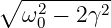 .
.
- Derive the condition ζ < 1∕
 for a nonzero-frequency displacement peak.
- Show that the velocity-amplitude response is maximized at ω0.
- Derive the average power formula and show that power is maximized at ω0.
- Derive the exact half-power frequencies and show that Δω = 2γ.
- Show that ω−ω+ = ω02.
- Derive Q = ω0∕(2γ) = mω0∕b from the bandwidth.
- Derive the beat solution for the undamped oscillator released from rest.
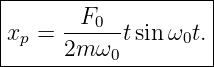
- Derive the secular solution xp = (F0∕2mω0)t sin ω0t at exact undamped resonance.
32 Summary
The driven damped oscillator obeys
After transients decay, the steady-state response is
The amplitude is
The phase lag is
The displacement-amplitude resonance occurs at
when that expression is real.
Power resonance occurs at
The half-power bandwidth is
and
In the undamped limit, near-resonant forcing produces beats, while exact resonance produces
secular growth:
M06-04 extends linear oscillation theory from one coordinate to multiple coupled coordinates and
introduces normal modes.
References
References
[1] PhysicsLibrary, M06-02, Damped Harmonic Motion.
[2] PhysicsLibrary, M06-01, Simple Harmonic Motion.
[3] A. P. French, Vibrations and Waves, W. W. Norton, 1971.
[4] J. R. Taylor, Classical Mechanics, University Science Books, 2005.








![x = e−γt[C cosω t + D sin ω t],
h d d](https://images.physicslibrary.org/cache/objects/1492/make4ht/DrivenHarmonicMotionAndResonance12x.png)



















![[ ]
xss(t) = Re X^ei ωt .](https://images.physicslibrary.org/cache/objects/1492/make4ht/DrivenHarmonicMotionAndResonance42x.png)


![|--------−γt---------------------------------------|
-x(t)-=-e---[C-cosωdt-+-D--sin-ωdt] +-X-cos(ωt-−--δ).-|](https://images.physicslibrary.org/cache/objects/1492/make4ht/DrivenHarmonicMotionAndResonance46x.png)














































![|--------------------------------|
| F0∕m |
x (t) = --2----2 [cos ωt − cosω0t].|
-------ω-0 −-ω--------------------](https://images.physicslibrary.org/cache/objects/1492/make4ht/DrivenHarmonicMotionAndResonance143x.png)










![|--------------------------|
xss-=-X-(ω-)cos[ωt-−-δ(ω)].-](https://images.physicslibrary.org/cache/objects/1492/make4ht/DrivenHarmonicMotionAndResonance164x.png)