Calculus of Variations: Several Dependent Variables and Vector Functionals

(Topic)

Calculus of Variations: Several Dependent Variables and Vector Functionals

The scalar calculus of variations developed in CV01–CV06 studies a single unknown function y(x). Many physical systems, however, have several coordinates evolving together. A double pendulum needs more than one angle, a spacecraft attitude model has several generalized coordinates, and even a simple pair of coupled masses requires two displacement functions.

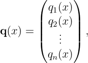
The natural variational unknown is then a vector-valued function

( q (x)) | 1 | | q2(x)| q(x) = |( ... |) , qn(x)

(1)

and the scalar functional becomes

|------∫--b--------------| J [q] = F (x,q,q ′) dx.| ---------a----------------

(2)

The functional still returns one real number, but it now evaluates an entire vector path. The corresponding stationarity condition is not one differential equation but a coupled system of Euler–Lagrange equations, one for each component of q [1, 2, 3].

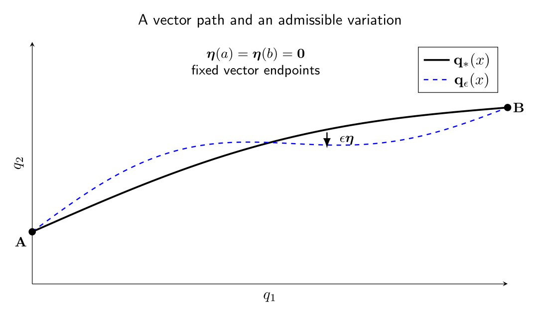
Figure. A vector-valued candidate path q_∗(x) and a nearby varied path q_𝜖(x) = q_∗(x) + 𝜖η(x). The variation η has one component for each dependent variable.

1 Learning objectives

After completing CV07, the reader should be able to

formulate a first-order variational problem with several dependent variables;
construct a vector variation q_𝜖 = q + 𝜖η;
derive the vector first-variation formula;
integrate by parts component by component;
use independent test-function components to obtain the coupled Euler–Lagrange equations;
express the result in component, vector, and matrix notation;
recognize generalized momenta in multi-degree-of-freedom mechanics;
derive the equations of a coupled quadratic system;
interpret vector endpoint conditions; and
distinguish coupling of equations from coupling of variations.

2 From one dependent variable to many

For one unknown function, the standard first-order functional is

∫ b ′ J[y] = F (x,y,y )dx. a

(3)

For n unknown functions, write

T ′ ′ ′T q = (q1,...,qn) , q = (q1,...,qn ) .

(4)

The integrand can depend on every coordinate and every derivative:

′ ′ F = F (x,q1,...,qn,q1,...,qn).

(5)

The functional is therefore

∫ b J [q1,...,qn ] = F(x,q1,...,qn,q1′,...,q′n) dx. a

(6)

The notation J[q] is shorter, but it is essential to remember that J still maps an admissible function or vector of functions to a scalar.

3 The admissible vector class

For fixed vector endpoints, a typical admissible class is

{ 1 n } 𝒜 = q ∈ C ([a,b];ℝ ) : q(a ) = A, q(b) = B .

(7)

Equivalently, each component satisfies

qi(a) = Ai, qi(b) = Bi, i = 1,...,n.

(8)

A vector-valued admissible path is therefore not a new kind of functional object; it is simply an ordered collection of admissible component functions. What changes is that the integrand can couple the components.

For example,

1- ′2 ′2 k- 2 F = 2(q1 + q2 ) + 2(q1 − q2)

(9)

cannot be separated into a term involving only q₁ plus a term involving only q₂. The difference q₁ − q₂ couples the two coordinates.

4 Vector variations

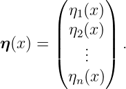
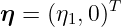
Let q_∗(x) be a candidate stationary path. Introduce a vector test function

( ) | η1(x)| | η2(x)| η(x) = |( ... |) . ηn(x )

(10)

The varied family is

|----------------------| -q𝜖(x) =-q∗(x) +-𝜖η(x).-

(11)

Componentwise,

qi,𝜖(x ) = qi,∗(x ) + 𝜖ηi(x).

(12)

Differentiating with respect to x gives

q′𝜖 = q′∗ + 𝜖η′.

(13)

For fixed endpoints,

|------------------------| |η(a ) = 0, η (b) = 0, | -------------------------

(14)

which means

η (a) = η(b) = 0 for every i. i i

(15)

The key new freedom is that the components of η can be chosen independently. We can perturb only q₁, only q₂, or any combination. That independence is what ultimately produces one Euler–Lagrange equation per component.

5 Scalarizing the vector problem

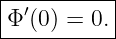
As in CV02, define the ordinary one-variable function

Φ(𝜖) = J[q∗ + 𝜖η].

(16)

If q_∗ is stationary, then for every admissible vector direction η,

|----------| |Φ′(0) = 0.| ------------

(17)

The first variation is

| -d- || δJ [q ∗;η] = d𝜖J [q ∗ + 𝜖η ]| . 𝜖=0

(18)

This is still a directional derivative of the functional. The only change is that the direction is vector-valued.

6 Deriving the vector first variation

Write

∫ b ′ ′ J [q 𝜖] = F (x,q ∗ + 𝜖η, q∗ + 𝜖η )dx. a

(19)

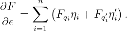
Assuming the regularity needed to differentiate under the integral sign,

∫ b || δJ = ∂-F (x,q∗ + 𝜖η,q ′∗ + 𝜖η ′)| dx. a ∂𝜖 |𝜖=0

(20)

The multivariable chain rule gives

n ∂F-- ∑ ( ′) ∂𝜖 = Fqiηi + Fq′iη i . i=1

(21)

Therefore

|-----------∫------------------------| | b∑ n ( ′) | |δJ[q∗;η] = Fqiηi + Fq′iη i dx.| -------------a--i=1--------------------

(22)

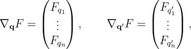
Using gradient notation,

( F ) ( F ′) | q.1| | .q1| ∇qF = ( .. ) , ∇q ′F = ( .. ) , Fqn Fq′ n

(23)

so the same result is

|-----∫-b----------------------------| δJ = [(∇ F )Tη + (∇ ′F)T η′] dx.| | a q q | --------------------------------------

(24)

The transpose simply represents the Euclidean dot product.

7 Integration by parts component by component

For each component,

∫ b ∫ b F ′η ′dx = [F ′η ]b− -d-F ′η dx. a qi i qi i a a dx qi i

(25)

Summing from i = 1 to n,

δJ	= _a^b	(26)
	+ ∫ _a^b ∑ _i=1ⁿ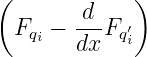η_i dx.	(27)

In vector notation,

|---------------------∫--[----------------]--------| | [ T ]b b -d- T | |δJ = (∇q ′F ) η a + ∇qF − dx ∇q ′F η dx. | -----------------------a---------------------------|

(28)

For fixed endpoints, η(a) = η(b) = 0, so the boundary term vanishes.

8 Why one vector integral gives n equations

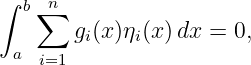
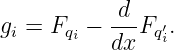
After the boundary term is removed, stationarity requires

∫ b∑n gi(x )ηi(x) dx = 0, a i=1

(29)

where

d gi = Fqi − ---Fq′i. dx

(30)

Now choose a variation having only its first component nonzero:

η = (η1,0,...,0)T.

(31)

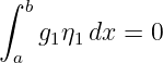
Then

∫ b g η dx = 0 a 1 1

(32)

for every admissible scalar test function η₁. The Fundamental Lemma gives

g = 0. 1

(33)

Repeat with

η = (0,η2,0,...,0)T,

(34)

and obtain g₂ = 0. Continuing through all components gives

gi = 0, i = 1,...,n.

(35)

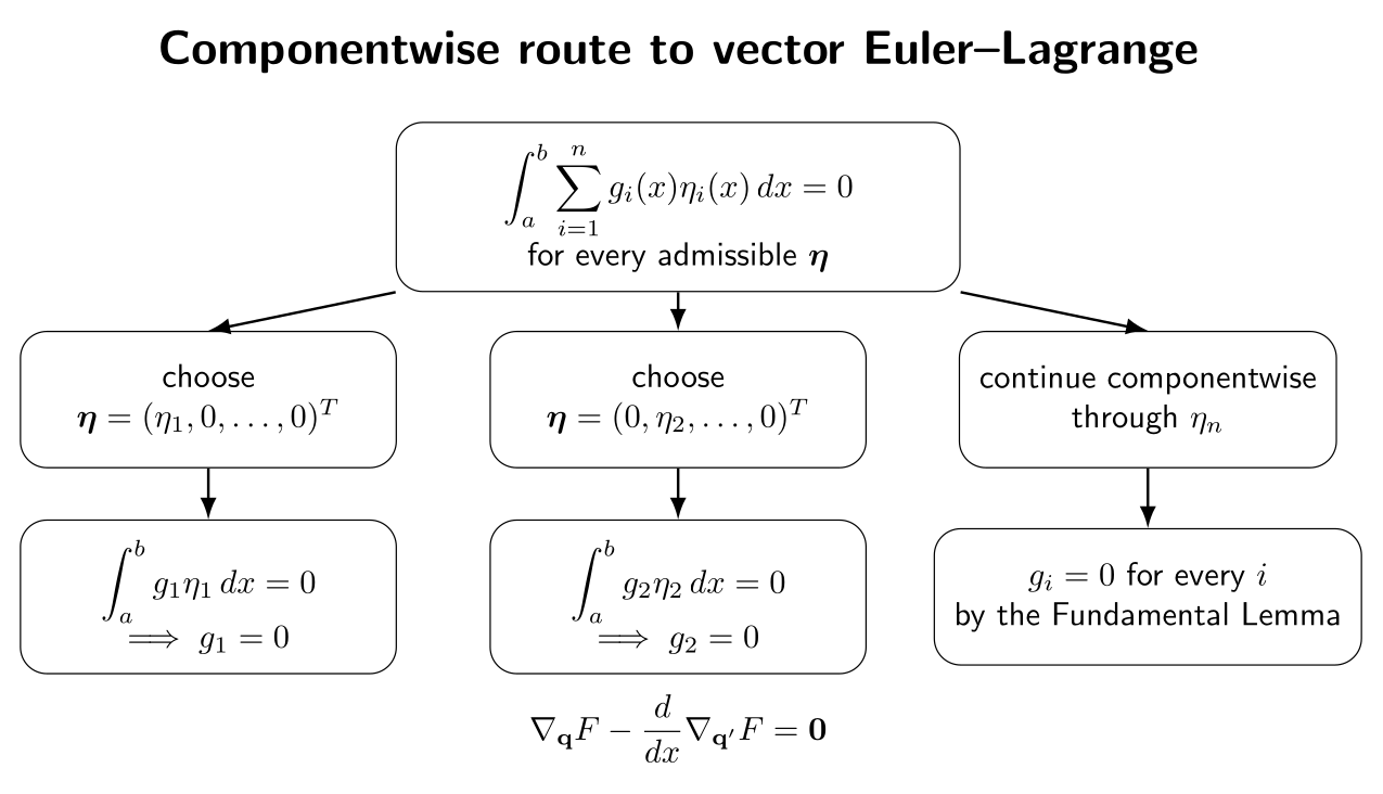
Figure. The vector Fundamental-Lemma step. Because each component of the test function can be selected independently, the single scalar stationarity condition yields one Euler–Lagrange equation for every dependent variable.

9 The vector Euler–Lagrange theorem

theorem. Let

∫ b ′ J[q] = a F (x,q,q ) dx,

(36)

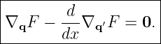
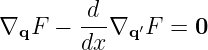
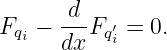
where F is sufficiently smooth and q_∗ ∈ C²([a,b]; ℝⁿ) is a stationary curve with fixed endpoints. Then each component satisfies

|---------------------------------| | -d- | Fqi − dx Fq′i = 0, i = 1,...,n. | -----------------------------------

(37)

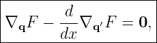
Equivalently,

|--------------------| ∇ F − -d-∇ ′F = 0.| --q-----dx---q--------

(38)

This vector equation is shorthand for n scalar differential equations. It does not mean that the equations are independent. If F couples the coordinates, the resulting equations are coupled as well.

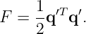
10 Example 1: vector Dirichlet energy and a straight path

Consider

∫ 1- b ′ 2 J[q] = 2 ∥q (x )∥ dx a

(39)

with fixed vector endpoints

q(a) = A, q (b) = B.

(40)

The integrand is

1 ′T ′ F = -q q . 2

(41)

Hence

∇qF = 0, ∇q ′F = q′.

(42)

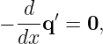
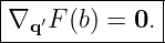
The vector Euler–Lagrange equation becomes

− -d-q′ = 0, dx

(43)

|-′′-----| -q--=-0.-|

(44)

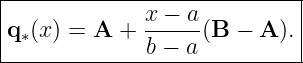
Integrating twice,

q(x) = C1x + C2.

(45)

Using the two vector endpoint conditions gives

|----------------------------| | x − a | |q∗(x) = A + b-−-a(B − A ).| -----------------------------

(46)

This is the affine parameterization of the straight segment from A to B.

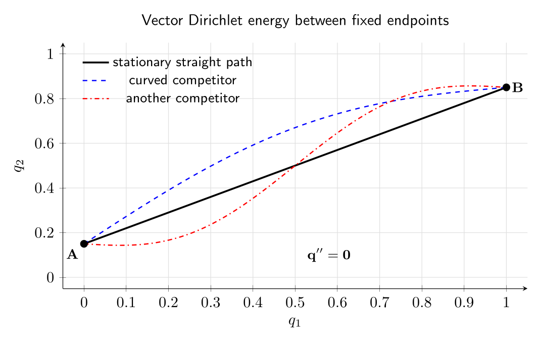
Figure. Several vector-valued paths joining the same endpoints in the plane. The stationary path for the quadratic vector Dirichlet energy is the straight segment, corresponding to q′′ = 0.

10.1 Why this is more than two separate scalar problems

For this particular integrand,

F = 1-q′2 + 1-q′2+ ⋅⋅⋅ + 1-q′2, 2 1 2 2 2 n

(47)

so the components decouple. Each equation is simply

′′ qi = 0.

(48)

That is a special case. The next example shows genuine coupling.

11 Example 2: a coupled quadratic variational problem

Consider two dependent variables and

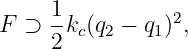
∫ b[ 1 1 1 1 1 ] J [q1,q2] = -m1q ′21 + --m2q2′2− -k1q21 − --k2q22 − -kc(q2 − q1)2 dx. a 2 2 2 2 2

(49)

Here m₁,m₂ > 0 and k₁,k₂,k_c ≥ 0. The k_c term couples the coordinates. For q₁,

Fq1 = − k1q1 + kc(q2 − q1), Fq′ = m1q ′1. 1

(50)

Therefore

− k1q1 + kc(q2 − q1) − m1q ′′= 0, 1

(51)

|------------------------------| |m q′′+ (k + k )q − k q = 0.| ---1-1-----1---c--1----c-2-----

(52)

For q₂,

Fq2 = − k2q2 − kc(q2 − q1), Fq′ = m2q ′2. 2

(53)

Hence

|------------------------------| |m2q ′′+ (k2 + kc)q2 − kcq1 = 0.| -----2-------------------------

(54)

The pair forms a coupled differential system.

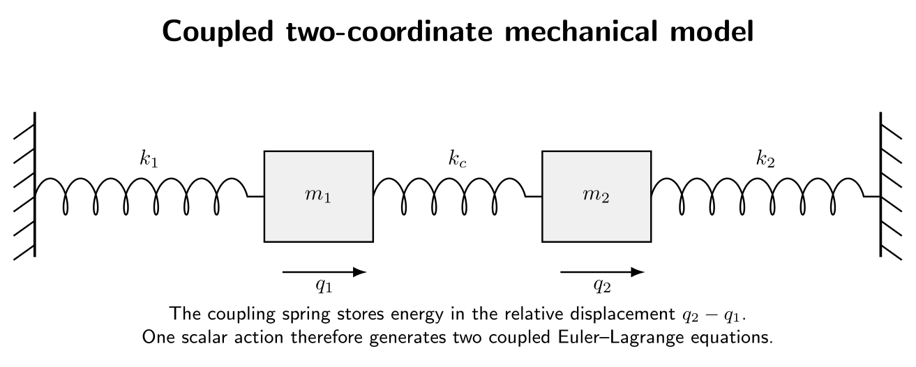
Figure. A mechanical interpretation of the coupled quadratic functional. The middle spring depends on the relative displacement q₂ − q₁, so varying either coordinate changes the coupling energy and therefore both Euler–Lagrange equations.

12 Matrix form of the coupled system

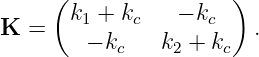
Define

( ) ( ) q1 m1 0 q = q2 , M = 0 m2 ,

(55)

and

( ) k1 + kc − kc K = − kc k2 + kc .

(56)

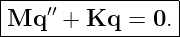
Then the two Euler–Lagrange equations become

|---′′-----------| -Mq---+-Kq--=--0.-

(57)

This is the standard matrix form of a linear multi-degree-of-freedom system. Its normal modes arise from the generalized eigenvalue problem

Kv = ω2Mv,

(58)

which belongs to vibration theory rather than to the derivation of the Euler–Lagrange equations themselves. The important variational lesson is that a single scalar action produces the full coupled matrix equation.

13 General multi-degree-of-freedom mechanics

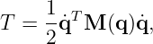
In mechanics, replace x by time t and let

T q(t) = (q1(t),...,qn(t))

(59)

be generalized coordinates. Hamilton’s principle uses the action

∫ t1 S [q ] = L (t,q, ˙q) dt. t0

(60)

Applying the vector Euler–Lagrange result gives

|---(----)-----------------------------| |-d ∂L- ∂L- | |dt ∂ ˙q − ∂q = 0, i = 1,...,n. | --------i-------i----------------------

(61)

These are Lagrange’s equations of the second kind [4, 5]. CV14 will develop Hamilton’s principle as a mechanics topic in its own right; CV07 is establishing the vector variational machinery needed for that step.

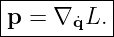
14 Generalized momentum becomes a vector

Define the generalized momentum components

pi = ∂L-. ∂ ˙qi

(62)

Collecting them gives

|----------| |p = ∇ ˙qL. | -----------

(63)

The Euler–Lagrange equations can then be written

˙p = ∇qL.

(64)

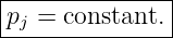
If a coordinate q_j is cyclic, then

∂L-- ∂qj = 0,

(65)

so its conjugate momentum satisfies

|p-=--constant.| --j-------------

(66)

Thus the scalar cyclic-coordinate result from CV06 extends componentwise to multi-coordinate systems.

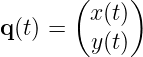
15 Example 3: planar particle in a potential

Let

( ) x(t) q(t) = y(t)

(67)

and take

L = 1m (˙x2 + ˙y2) − V(x, y). 2

(68)

For x,

∂L ∂L ∂x- = − Vx, ∂x˙= m ˙x,

(69)

m ¨x + Vx = 0.

(70)

Similarly,

m ¨y + Vy = 0.

(71)

Together,

|---------------| m-¨q-+-∇V---=-0.-|

(72)

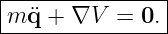
Since force is F = −∇V , this is

m ¨q = F.

(73)

The familiar vector form of Newton’s second law therefore emerges directly from a vector variational principle.

16 Vector endpoint conditions

The integration-by-parts boundary term for a vector functional is

[ T ]b (∇q ′F ) η a .

(74)

For fixed vector endpoints, every component of η vanishes and there is no natural boundary condition.

If instead the terminal vector q(b) is completely free while b is fixed, then η(b) is arbitrary. Stationarity requires

|-------------| ∇q ′F(b) = 0. | ---------------

(75)

Componentwise,

F ′(b) = 0, i = 1,...,n. qi

(76)

More complicated partial endpoint freedom is handled by allowing only the corresponding components or tangent directions of η to vary. This is the vector extension of the natural-boundary and transversality ideas from CV05.

17 Coupling of equations versus independence of variations

Two statements that sound contradictory are both true:

the components q_i may be strongly coupled through F;
the variation components η_i may still be chosen independently when the admissible class places no constraint coupling them.

The first statement concerns the physical or mathematical model. The second concerns the allowable perturbations used to test stationarity.

For the coupled oscillator,

1- 2 F ⊃ 2kc(q2 − q1) ,

(77)

so the final equations are coupled. Nevertheless, choosing

T η = (η1,0)

(78)

is legitimate under unconstrained fixed-endpoint variations, and it isolates the first Euler–Lagrange equation in the proof.

If the admissible class itself imposes a relation such as

G (q1,q2) = 0,

(79)

then the variations are no longer independent. That is a constrained variational problem and is postponed to CV09 and CV15.

18 Several cyclic coordinates

Suppose

F = F (x,q,q ′)

(80)

is independent of a subset of the coordinates, for example

Fq2 = Fq4 = 0.

(81)

Then the corresponding Euler–Lagrange equations give

Fq′ = C2, Fq′ = C4. 2 4

(82)

Each cyclic coordinate produces its own first integral. This is one reason symmetry becomes especially powerful in multi-degree-of-freedom systems: a single model can possess several conserved generalized momenta.

19 The Hessian with respect to derivatives

For one dependent variable, the regularity of the Euler–Lagrange equation is connected with

Fy′y′.

(83)

For several dependent variables, the analogous object is the matrix

[ ∂2F ]n Hq ′q′ = ---′-′- . ∂qi∂qj i,j=1

(84)

If this matrix is nonsingular, the vector Euler–Lagrange equations can often be solved locally for the highest derivatives q′′. In mechanics, for a standard kinetic energy

T = 1-˙qTM (q)˙q, 2

(85)

this Hessian is closely related to the mass matrix. Singular Hessians occur in constrained or gauge-type systems and require additional theory.

CV07 uses only the classical regular case; the matrix viewpoint is introduced now so that the later mechanics and optimal-control entries have a natural language.

20 Necessary conditions are still only necessary

The vector Euler–Lagrange equations are stationarity conditions. A solution of

-d- ∇qF − dx ∇q ′F = 0

(86)

need not minimize the functional. It may be a maximum, saddle, or other stationary path. The second variation becomes a quadratic form in the vector variation η, and its classification involves matrix-valued coefficients. That analysis begins in CV11.

Existence is likewise separate. A formal solution of the coupled boundary value problem does not by itself prove that a minimizer exists in the chosen admissible function space.

21 Common mistakes

Mistake: treating J[q] as vector-valued. The path is vector-valued, but the functional considered here still returns one scalar.
Mistake: writing only one Euler–Lagrange equation for several dependent variables. There is one equation for each independent component.
Mistake: assuming coupled equations imply the test functions cannot be chosen componentwise. Coupling in F does not by itself restrict the admissible variations.
Mistake: differentiating F_{q_i′} only partially with respect to x. The derivative dF_{q_i′}∕dx is a total derivative along the path.
Mistake: confusing ∇_qF with a spatial gradient in physical space. It is the gradient of F with respect to its coordinate arguments q_i.
Mistake: forgetting that constraints can destroy componentwise independence of the variations.
Mistake: interpreting every stationary vector path as a minimum.

22 A practical vector Euler–Lagrange checklist

Given

∫ b J[q] = F (x,q,q ′) dx, a

(87)

use the following workflow:

List the dependent variables q₁,…,q_n.
State the admissible class and all endpoint or coupling constraints.
Introduce q_𝜖 = q + 𝜖η.
Determine which components of η are independent.
Compute F_{q_i} and F_{q_i′} for every component.
Form
$Fq − -d-Fq′ = 0. i dx i$
Collect the equations into vector or matrix form if useful.
Apply fixed, natural, or transversality endpoint conditions.
Inspect cyclic coordinates for first integrals from CV06.
Keep stationarity separate from minimum classification and existence.

23 Summary

For the vector functional

∫ b J[q] = F (x,q,q ′) dx, a

(88)

an admissible vector variation is

q𝜖 = q ∗ + 𝜖η.

(89)

The first variation is

∫ b[ T T ′] δJ = (∇qF ) η + (∇q ′F) η dx. a

(90)

After componentwise integration by parts and the Fundamental Lemma,

|--------------------| ∇qF − -d-∇q ′F = 0,| --------dx------------

(91)

or equivalently

|---------------------------------| | -d- | Fqi − dx Fq′i = 0, i = 1,...,n. | -----------------------------------

(92)

A single scalar functional can therefore generate an entire coupled system of differential equations. In mechanics this becomes the multi-coordinate form of Lagrange’s equations, while in geometry it governs vector-valued stationary paths. CV07E1 will practice coupled systems, and CV07E2 will apply the vector formulation to trajectory problems. CV08 next extends the variational machinery to functionals containing higher derivatives.

References

[1] I. M. Gelfand and S. V. Fomin, Calculus of Variations, Dover Publications, 2000.

[2] Bruce van Brunt, The Calculus of Variations, Springer, 2004.

[3] Robert Weinstock, Calculus of Variations with Applications to Physics and Engineering, Dover Publications, 1974.

[4] Cornelius Lanczos, The Variational Principles of Mechanics, 4th ed., Dover Publications, 1986.

[5] Herbert Goldstein, Charles Poole, and John Safko, Classical Mechanics, 3rd ed., Addison Wesley, 2002.

"Calculus of Variations: Several Dependent Variables and Vector Functionals" is owned by bloftin.
(view preamble)

Calculus of Variations: Several Dependent Variables and Vector Functionals