Calculus of Variations: Endpoints, Natural Boundary Conditions, and Transversality

The fixed-endpoint Euler–Lagrange theorem in CV04 used the condition

η(a) = η(b) = 0

(1)

at one decisive moment: it removed the boundary term produced by integration by parts. If an endpoint is free, that term does not disappear. Instead, it becomes an additional necessary condition.

That observation is the source of natural boundary conditions and transversality conditions; standard treatments derive both from the boundary part of the first variation [1, 2, 3]. The interior of a stationary curve is still governed by the Euler–Lagrange equation,

F − -d-F ′ = 0, y dx y

(2)

but the endpoint geometry determines what must happen at the boundary.

This distinction is essential in physics. A prescribed position is an essential or Dirichlet-type condition. A free position may instead force a conjugate momentum, slope, traction, or flux to vanish. If the endpoint is allowed to slide along a curve, the variational boundary term must vanish for every motion tangent to that curve. In geometrical optics and shortest-path problems this becomes an orthogonality condition. In mechanics it becomes a statement about canonical momentum and Hamiltonian. In optimal control the same structure reappears as terminal transversality conditions.

1 Learning objectives

After this entry, the reader should be able to

retain and interpret the boundary term in the first variation;
distinguish essential boundary data from natural boundary conditions;
derive the natural condition F_y′ = 0 at a fixed-x, free-y endpoint;
handle mixed endpoint conditions and endpoints free at one or both ends;
derive the full endpoint variation for a moving point (x,y);
explain the relation between the field variation η and the actual endpoint displacement;
derive the transversality condition for an endpoint constrained to a curve y = ψ(x) or, more generally, G(x,y) = 0;
prove that a shortest path to a smooth target curve meets that curve orthogonally;
include an endpoint cost Φ(x_b,y_b) and derive the resulting terminal conditions;
rewrite the endpoint term as pδy − H δx;
interpret the variational boundary conditions in classical mechanics; and
recognize why natural boundary conditions do not replace the Euler–Lagrange equation but supplement it.

2 The boundary term CV04 set to zero

For

∫ b J[y] = F (x,y,y′)dx, a

(3)

CV02 gave

∫ b δJ[y;η] = (Fy η + Fy′η ′)dx. a

(4)

Integration by parts gives

∫ b( ) b -d- δJ[y;η] = [Fy ′η]a + a Fy − dx Fy′ η dx.

(5)

For a stationary curve, the interior Euler–Lagrange equation makes the integral term vanish. What remains is

|------------------| δJ = [F ′η]b| ---boundary-----y--a-

(6)

when the independent-variable endpoints a and b themselves are fixed.

The endpoint assumptions now determine what follows.

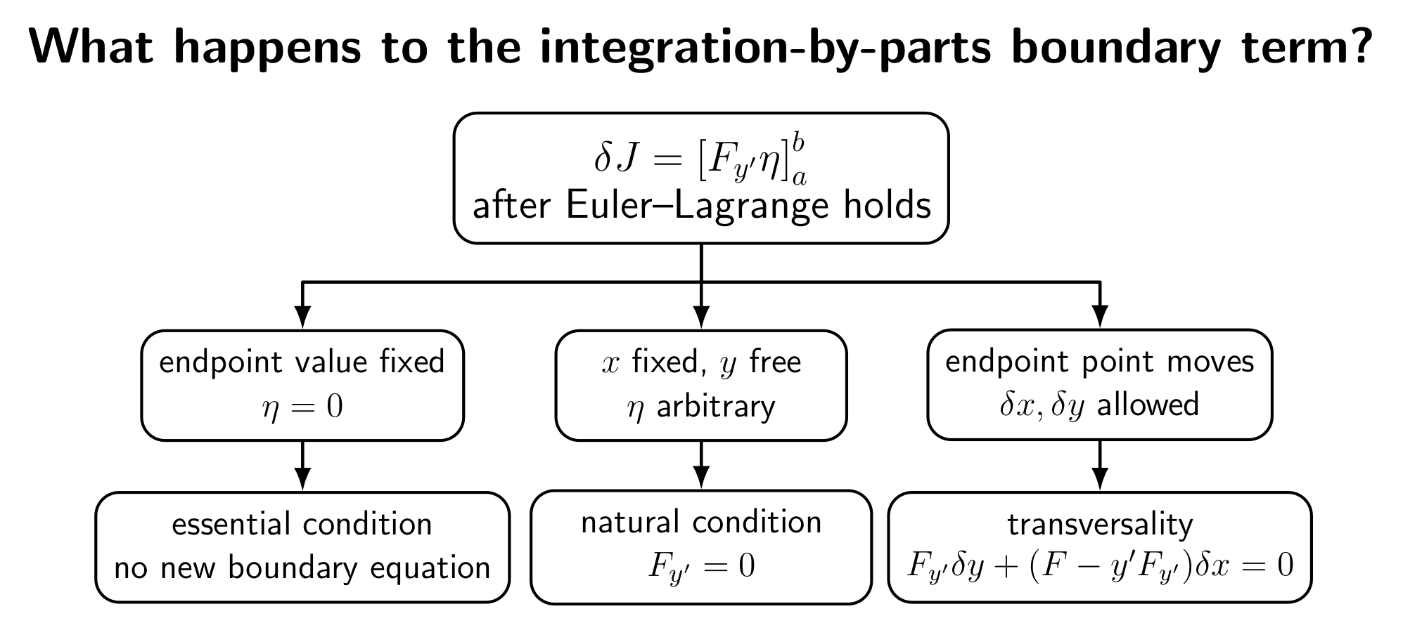
Figure. The same integration-by-parts boundary term leads to different necessary conditions depending on what is prescribed at the endpoint. Fixed endpoint values force η = 0; free endpoint values leave η arbitrary and therefore force F_y′ = 0.

3 Essential and natural boundary conditions

Suppose the endpoint abscissas a and b are fixed.

3.1 Fixed endpoint value: an essential condition

y(b) = B

(7)

is prescribed, then every admissible variation must satisfy

η(b) = 0.

(8)

The boundary term vanishes because admissibility removes that degree of freedom. The condition y(b) = B is therefore imposed directly on the admissible class. In the language of boundary-value problems, this is an essential or Dirichlet-type boundary condition.

3.2 Free endpoint value: a natural condition

Now suppose x = b is fixed but the value y(b) is not prescribed. Then η(b) is arbitrary. If the left endpoint is fixed, η(a) = 0, and the boundary contribution reduces to

′ Fy ′(b,y(b),y (b))η (b).

(9)

Stationarity requires this to vanish for every allowed value of η(b). Therefore

|--------------------| Fy ′(b,y(b),y′(b)) = 0.| ----------------------

(10)

This is the classical natural boundary condition at a free terminal value.

Exactly the same argument at the left endpoint gives

|---------------------| F ′(a,y(a),y′(a)) = 0 | --y-------------------

(11)

when y(a) is free and a is fixed.

If both endpoint values are free while a and b remain fixed, then

Fy′(a ) = 0, Fy′(b) = 0.

(12)

4 The natural-boundary theorem

Theorem: fixed-x, free-y endpoint. Let

∫ b J[y] = F (x,y,y′)dx, a

(13)

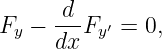
with F ∈ C² on a region containing the relevant curve. Suppose y_∗ ∈ C²([a,b]) is a weak local extremum, y(a) = A is fixed, and y(b) is free. Then y_∗ satisfies

Fy − d-Fy′ = 0 for a < x < b, dx

(14)

and the natural terminal condition

F ′(b,y (b),y′(b)) = 0. y ∗ ∗

(15)

Proof. Choose first variations with compact support in (a,b). The Fundamental Lemma gives the Euler–Lagrange equation in the interior exactly as in CV04. After imposing that equation, the full first variation is

δJ = [Fy ′η]b. a

(16)

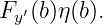
Because y(a) is fixed, η(a) = 0. Since y(b) is free, η(b) may be chosen arbitrarily. Hence

Fy′(b)η (b) = 0

(17)

for every real value of η(b), which implies F_y′(b) = 0. □

The proof is short because all the conceptual work was already done in CV02, CV03, and CV04. The new point is simply that endpoint freedom creates an additional admissible variation.

5 Example: a free endpoint selects the slope

Consider

∫ 1 1( ′2 2) J[y] = -- (y ) + y dx, 0 2

(18)

subject to

y(0) = A,

(19)

while y(1) is free.

Here

F = 1((y′)2 + y2), F = y, F ′ = y′. 2 y y

(20)

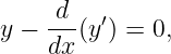
The Euler–Lagrange equation is

d ′ y − dx-(y ) = 0,

(21)

y′′ = y.

(22)

The natural boundary condition at x = 1 is

y′(1) = 0.

(23)

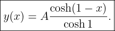
The solution of y′′ = y satisfying y(0) = A and y′(1) = 0 is

|----------------------| | cosh(1 − x) | |y(x) = A ------------.| -------------cosh1-----

(24)

Thus a free terminal value does not mean that “nothing is specified” at the right boundary. The variational principle itself supplies the missing condition.

6 Mixed boundary conditions

The endpoint conditions can be mixed independently.

For example,

y (a ) = A, y(b) free

(25)

gives

η(a) = 0, Fy ′(b) = 0.

(26)

Conversely,

y (a ) free, y(b) = B

(27)

leads to

Fy′(a ) = 0, η(b) = 0.

(28)

This is the simplest manifestation of a general principle:

A prescribed endpoint coordinate removes a variation; a free endpoint coordinate produces a variational boundary equation.

7 Moving endpoints require a new calculation

So far the endpoint abscissas a and b have been fixed. Transversality arises when an endpoint may move in the (x,y) plane.

Consider the terminal point

B = (b,y(b)).

(29)

Let its actual infinitesimal displacement be

(δxb,δyb).

(30)

There is an important distinction between δy_b and the field variation η(b). When the endpoint moves horizontally, part of its vertical change comes simply from moving along the unperturbed curve.

To first order,

|----------------------| |δyb = η(b) + y′(b)δxb. | -----------------------

(31)

Therefore

η(b) = δyb − y′(b)δxb.

(32)

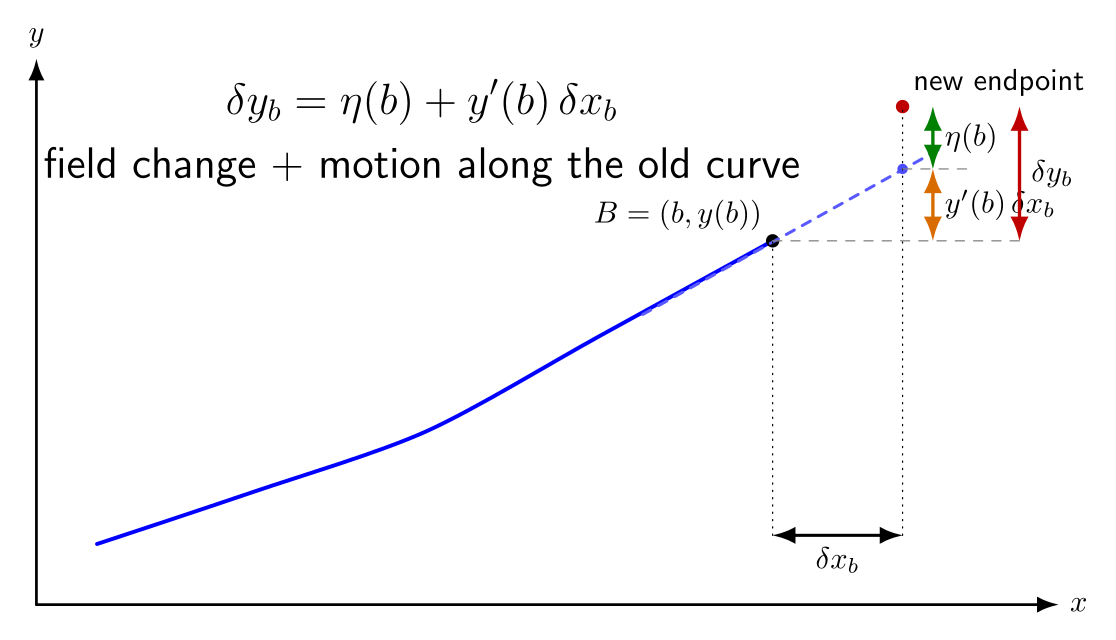
Figure. Geometry of a moving terminal endpoint. The total vertical displacement δy_b contains both the fixed-x field variation η(b) and the vertical change y′(b)δx_b caused by shifting the endpoint horizontally along the original curve.

8 Derivation of the moving-endpoint boundary term

For clarity, let the left endpoint remain fixed and allow only the upper endpoint to move. The first-order change in the integral receives two boundary contributions.

First, integration by parts gives

Fy′(b)η(b).

(33)

Second, changing the upper limit contributes

F (b)δxb.

(34)

Hence, after the Euler–Lagrange equation has removed the interior term,

δJb = Fy′η(b) + Fδxb.

(35)

Insert

′ η(b) = δyb − y δxb.

(36)

Then

δJ_b	= F_y′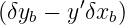 + Fδx_b	(37)
	= F_y′δy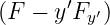_b + δx_b.	(38)

Thus the universal terminal boundary form is

|------------------------------| |δJ = F ′ δy + (F − y′F ′)δx .| ---b----y---b-----------y----b--

(39)

If both endpoints move, the complete boundary contribution can be written compactly as

|--------------------------------------| |δJ = [F ′ δy + (F − y ′F ′)δx ]b . ---boundary-----y---------------y----a--

(40)

Here the bracket means terminal contribution minus initial contribution.

9 Special cases of the moving-endpoint formula

The general boundary form immediately contains several important cases.

9.1 Fixed x, free y

Set

δx = 0,

(41)

while δy is arbitrary. Then

Fy′ = 0,

(42)

which recovers the natural boundary condition.

9.2 Free x, fixed endpoint value y

If the endpoint may slide horizontally while its vertical coordinate is fixed, then

δy = 0

(43)

and stationarity requires

|--------------| |F − y′Fy′ = 0.| ----------------

(44)

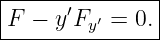
9.3 Endpoint completely free in the plane

If δx and δy are independently arbitrary, then both coefficients must vanish:

Fy ′ = 0, F − y ′Fy′ = 0.

(45)

Consequently

F = 0

(46)

at the endpoint as well. This strong condition is one reason fully free endpoints are often supplemented by terminal costs or geometric constraints.

10 Endpoint constrained to a curve: transversality

Suppose the terminal endpoint must lie on a smooth target curve

y = ψ (x).

(47)

An allowed endpoint displacement must be tangent to this curve, so

′ δyb = ψ (b)δxb.

(48)

Substitute this relation into the terminal boundary form:

δJ_b	= F_y′ψ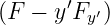′δx_b + δx_b	(49)
	= δx_b.	(50)

Because motion along the target curve is arbitrary,

|--------------------| |F + (ψ ′ − y′)F ′ = 0 ---------------y------

(51)

at the terminal point.

This is a classical transversality condition.

11 Coordinate-free geometric form

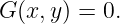
A target curve can also be written implicitly as

G (x, y) = 0.

(52)

An allowed tangent displacement satisfies

Gx δx + Gyδy = 0.

(53)

Define the boundary covector

b = (F − y′Fy′, Fy′).

(54)

Stationarity requires

b ⋅ (δx, δy) = 0

(55)

for every tangent displacement to the target curve. Therefore b must be normal to the target curve:

|----------------------| |(F − y′Fy′, Fy′) ∥ ∇G.| ------------------------

(56)

This is the geometric content of transversality. The variational boundary covector must annihilate every allowed endpoint motion.

12 Example: shortest path to a target curve

For planar arc length,

∫ b∘ ------′2- J [y] = 1 + (y ) dx, a

(57)

∘ -----′-2- -----y′----- F = 1 + (y ) , Fy ′ = ∘ 1 + (y ′)2.

(58)

Let the terminal endpoint lie on

y = ψ (x).

(59)

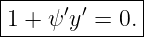
The transversality condition is

′ ∘ ------′-2 ′ ′ ∘---y------ 1 + (y ) + (ψ − y ) 1 + (y′)2 = 0.

(60)

Multiply through by ---------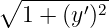
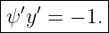
∘ 1 + (y′)2 :

′ 2 ′ ′ ′2 1 + (y ) + ψ y − (y) = 0.

(61)

Therefore

|------------| 1 + ψ ′y ′ = 0. --------------

(62)

If both slopes are finite,

|----------| | ′ ′ | ψ--y-=-−-1.-

(63)

This is exactly the condition for perpendicular tangent lines. Thus:

The shortest curve from a fixed point to a smooth target curve meets the target curve orthogonally.

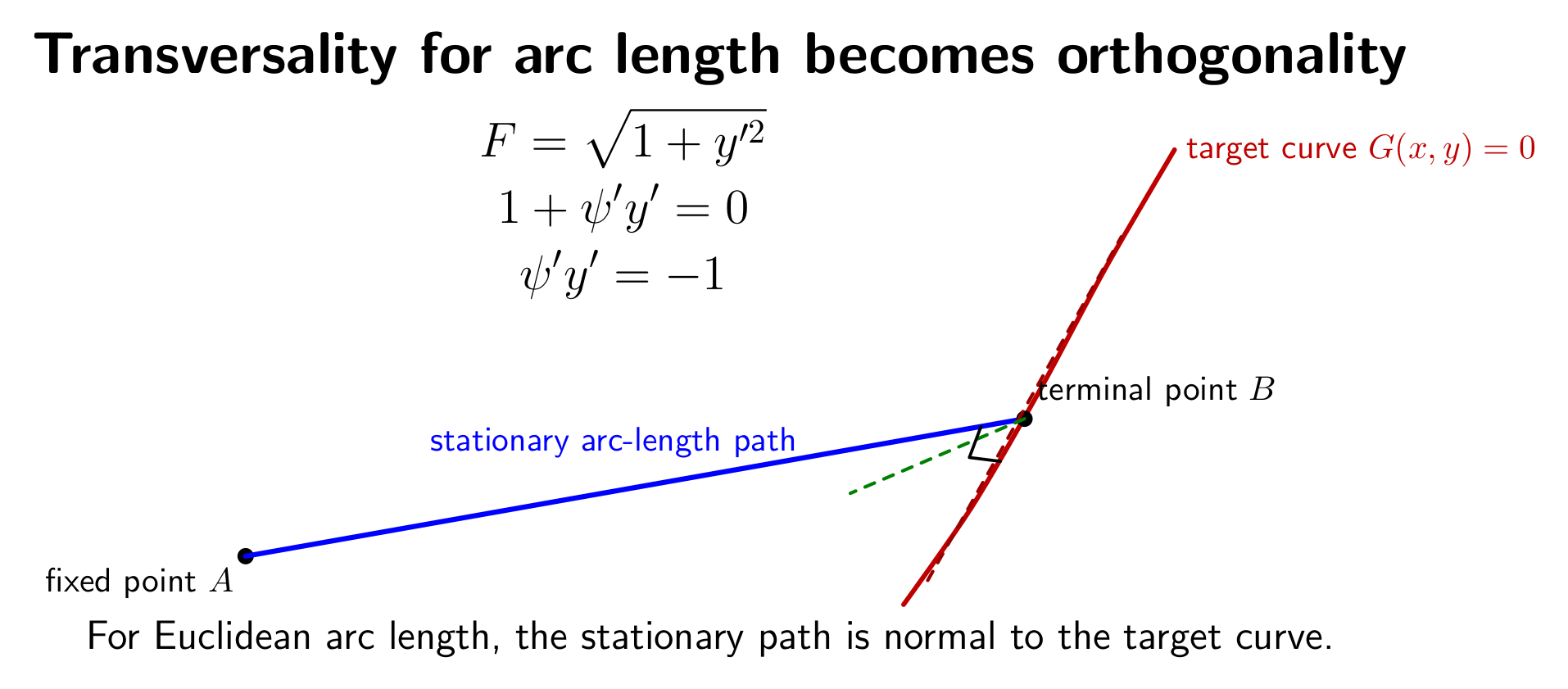
Figure. For the arc-length functional, the transversality condition says that the stationary path reaches the target curve at right angles. The familiar Euclidean orthogonality rule is therefore a variational boundary condition.

12.1 Straight target line

If the target is

y = mx + c,

(64)

then ψ′ = m and

′ 1- y = − m .

(65)

Because the Euler–Lagrange equation for arc length makes the stationary path a straight line, the entire problem reduces to the elementary geometric result: the shortest line segment to a line is the perpendicular segment.

13 Endpoint costs

Many physics and control problems include a terminal contribution in addition to the integral. Consider

∫ b ′ 𝒥 [y] = a F(x,y, y) dx + Φ(b,y(b)),

(66)

where the terminal point may move.

The variation of the endpoint cost is

δ Φ = Φx δxb + Φyδyb.

(67)

Adding this to the moving-endpoint boundary form gives

δ𝒥 = (F ′ + Φ )δy + (F − y′F ′ + Φ )δx . b y y b y x b

(68)

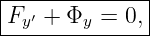
If the terminal point is completely free, the two independent terminal conditions are

|--------------| |Fy′ + Φy = 0, | ---------------

(69)

and

|--------------------| |F − y′Fy ′ + Φx = 0.| ---------------------

(70)

If the terminal point is constrained to a curve, only the component along the allowed tangent displacement must vanish.

14 Example: an endpoint spring gives a Robin condition

Consider

∫ [ ] 1 1- ′2 k- 2 𝒥 [y] = 2(y ) + V (y) dx + 2 (y(1) − Y ) , 0

(71)

with y(0) fixed and y(1) free.

The integral gives

′ Fy ′ = y .

(72)

The terminal cost has

Φy = k (y (1 ) − Y ).

(73)

Therefore the natural terminal condition becomes

|------------------------| |y′(1) + k (y (1 ) − Y ) = 0. --------------------------

(74)

This is a Robin-type boundary condition: the boundary value and its derivative are coupled. Physically, the terminal spring converts endpoint displacement into a boundary force.

15 Momentum and Hamiltonian form of the boundary term

Define the momentum-like quantity

p = Fy ′

(75)

and define

′ H = y p − F.

(76)

Then

F − y′Fy′ = − H.

(77)

The moving-endpoint boundary term becomes

|--------------------| |δJ = pδy − H δx .| ---b-------b-------b-

(78)

With an endpoint cost,

|------------------------------------| |δ𝒥b = (p + Φy )δyb + (− H + Φx)δxb. | -------------------------------------

(79)

This form is not merely elegant notation. It is the direct ancestor of terminal conditions in Hamiltonian mechanics and optimal control [4, 5, 6].

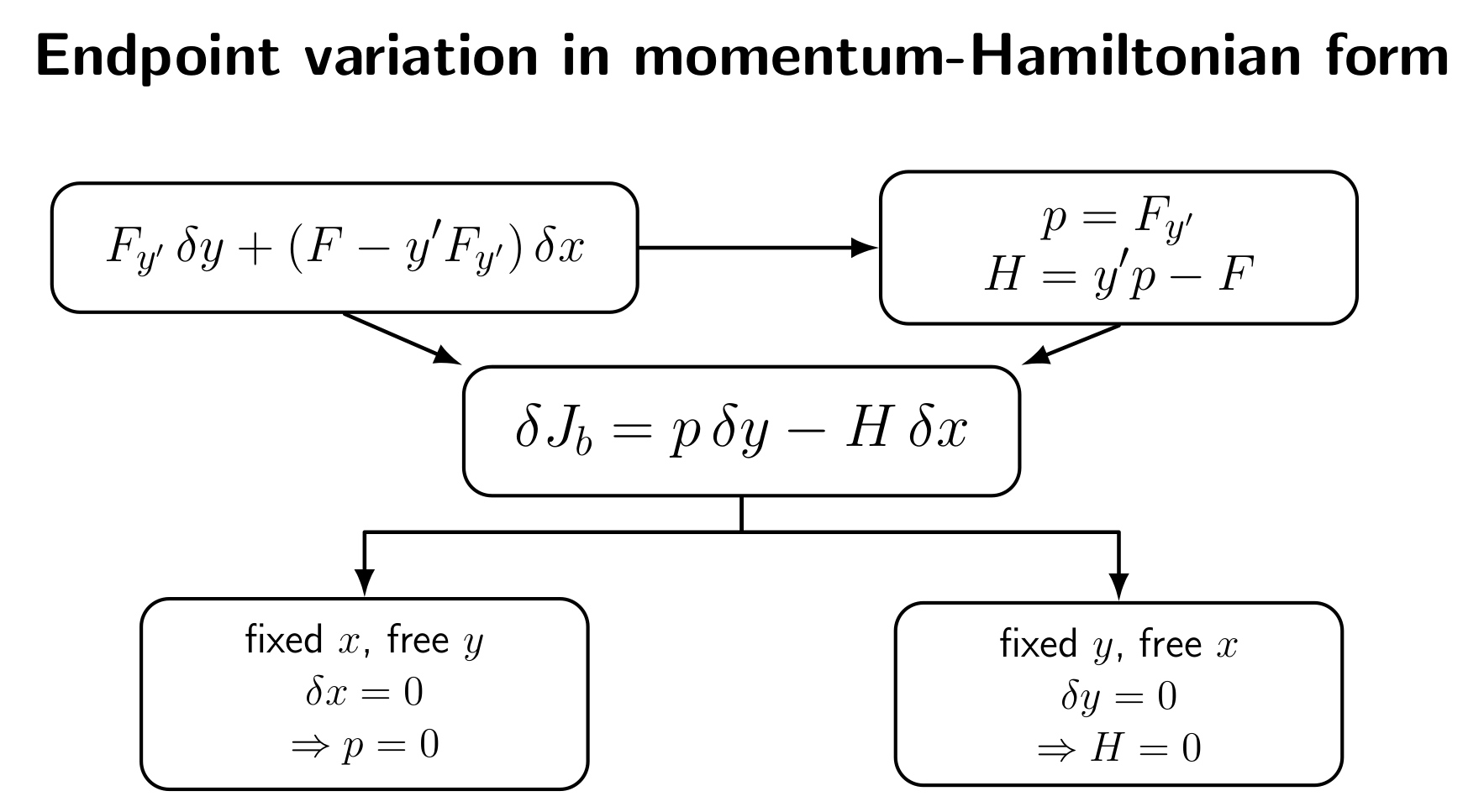
Figure. The endpoint one-form can be written in momentum-Hamiltonian variables. A free terminal configuration tests the coefficient of δy; a free terminal independent variable tests the coefficient of δx.

16 Mechanical interpretation

Let the independent variable be time and set

F = L(t,q, ˙q).

(80)

Then

∂L- p = ∂ ˙q

(81)

is the canonical momentum and

H = p˙q − L

(82)

is the Hamiltonian when the Legendre transformation is regular.

The terminal contribution to Hamilton’s principle is therefore

δSf = pf δqf − Hf δtf.

(83)

Several familiar terminal conditions follow immediately.

16.1 Fixed final time, free final coordinate

δtf = 0

(84)

while δq_f is arbitrary, then

|-------| pf = 0. | ---------

(85)

A free terminal coordinate forces the conjugate momentum to vanish unless some terminal interaction supplies an additional boundary contribution.

16.2 Free final time, fixed final coordinate

If the actual terminal coordinate is fixed,

δqf = 0,

(86)

while δt_f is arbitrary, then

|--------| |H = 0.| ---f-----

(87)

for an action with no terminal cost.

16.3 Terminal cost in mechanics

For

∫ tf S [q] = L (t,q, ˙q)dt + Φ (tf ,qf), t0

(88)

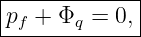
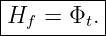
fully free terminal data give

|------------| |pf + Φq = 0,| --------------

(89)

and

|---------| Hf = Φt. | -----------

(90)

The sign of the Hamiltonian terminal equation depends on the convention used to define the Hamiltonian and the objective functional. With the mechanical Hamiltonian convention used above and the additive terminal cost written here, the formula is exactly as shown.

17 Why these are called natural boundary conditions

The adjective “natural” is used because these conditions are not imposed externally as part of the admissible class. They emerge from stationarity of the functional itself.

For a first-order scalar functional:

prescribing y is essential data;
leaving y free produces the natural quantity F_y′;
allowing x to move introduces the companion quantity F − y′F_y′;
constraining the endpoint geometrically requires the boundary covector to annihilate allowed tangent motions.

In elasticity and field theory, the same pattern produces tractions and fluxes. In mechanics it produces momenta. In weak formulations, natural boundary data appear automatically in the boundary terms generated by integration by parts [2, 3].

18 Natural conditions do not replace Euler–Lagrange

A frequent conceptual mistake is to treat the boundary condition as an alternative to the Euler–Lagrange equation. It is not.

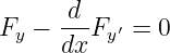
A stationary free-endpoint problem generally requires both

d Fy − ---Fy′ = 0 in the interior dx

(91)

and one or more endpoint conditions.

The interior equation determines the family of candidate extremals. The boundary conditions select which member of that family is compatible with the endpoint freedom and geometry.

19 Necessary still does not mean sufficient

Everything derived in this entry is a necessary condition for a sufficiently smooth local extremum under the stated hypotheses. A function can satisfy

F − -d-F ′ = 0 y dx y

(92)

and all natural or transversality conditions and still fail to minimize the functional.

Classification requires the second variation and the stronger conditions studied later in the course. Endpoint freedom changes the admissible perturbations, so second-variation theory must also respect the relevant boundary geometry.

20 Common misconceptions

20.1 Misconception 1: free endpoint means no boundary condition

The opposite is usually true. Freedom makes the endpoint variation arbitrary, which forces a natural boundary equation.

20.2 Misconception 2: η(b) = δy_b for a moving endpoint

Only when δx_b = 0. In general,

δyb = η(b) + y′(b)δxb.

(93)

This distinction is essential for deriving the correct transversality formula.

20.3 Misconception 3: the transversality condition is always orthogonality

Orthogonality occurs for special functionals such as Euclidean arc length. The general condition is

F ′δy + (F − y′F ′)δx = 0 y y

(94)

for every allowed endpoint displacement.

20.4 Misconception 4: F − y′F_y′ is always the physical energy

Not in an arbitrary variational problem. It equals −H after one defines H = y′F_y′− F. In mechanics that quantity becomes the Hamiltonian under the usual regularity assumptions.

20.5 Misconception 5: natural boundary conditions prove a minimum

They are necessary stationarity conditions, not sufficient classification criteria.

21 A compact endpoint-condition table


Endpoint freedom	Necessary boundary statement

x fixed, y prescribed	η = 0; no new natural condition

x fixed, y free	F_y′ = 0

y fixed, x free	F − y′F_y′ = 0

(x,y) completely free	F_y′ = 0 and F − y′F_y′ = 0

y = ψ(x)	F + (ψ′− y′)F_y′ = 0

G(x,y) = 0	(F − y′F_y′,F_y′) ∥∇G

free terminal point with Φ	F_y′ + Φ_y = 0, F − y′F_y′ + Φ_x = 0

22 Connection to the next entries

CV05 completes the endpoint layer of the basic Euler–Lagrange theory. The next main lesson, CV06, studies special forms of the integrand that produce first integrals and conservation-like quantities without solving the full second-order Euler–Lagrange equation directly.

In particular, when F has no explicit dependence on x, the quantity

F − y′F ′ y

(95)

that appeared here as a boundary coefficient also becomes constant along an extremal. That result is the Beltrami identity. The recurrence of the same quantity in both endpoint variation and first-integral theory is an early sign of the deeper Hamiltonian structure developed later in the course.

23 Summary

The first variation naturally separates into an interior term and a boundary term. Fixed endpoint values eliminate boundary variations by admissibility; free endpoint values turn those boundary variations into additional equations.

For fixed independent-variable endpoints,

δJ = [F ′η]b , boundary y a

(96)

so a free endpoint value gives the natural condition

Fy′ = 0.

(97)

When the endpoint itself moves in the (x,y) plane,

δJ = [F ′δy + (F − y ′F ′)δx]b. boundary y y a

(98)

An endpoint constrained to a curve must satisfy the corresponding transversality condition. For Euclidean arc length, this reduces to orthogonality between the stationary path and the target curve.

Finally, with

p = Fy′, H = y′p − F,

(99)

the boundary form becomes

δJb = pδy − H δx,

(100)

providing a direct bridge from classical calculus of variations to Hamiltonian mechanics and terminal conditions in optimal control.

References

[1] I. M. Gelfand and S. V. Fomin, Calculus of Variations, Dover Publications, 2000.

[2] Bruce van Brunt, The Calculus of Variations, Springer, 2004.

[3] Charles Fox, An Introduction to the Calculus of Variations, Dover Publications, 1987.

[4] Herbert Goldstein, Charles Poole, and John Safko, Classical Mechanics, 3rd ed., Addison Wesley, 2002.

[5] L. D. Landau and E. M. Lifshitz, Mechanics, 3rd ed., Course of Theoretical Physics, Vol. 1, Pergamon Press, 1976.

[6] Donald E. Kirk, Optimal Control Theory: An Introduction, Prentice-Hall, 1970.

"Natural Boundary Conditions Calculus of Variations: Endpoints" is owned by bloftin.
(view preamble)