Calculus of Variations: Constrained Variations and Isoperimetric Problems
The Euler–Lagrange equation developed in CV04 assumes that the admissible function may be
perturbed in every sufficiently small endpoint-preserving direction. Many important variational
problems impose an additional global condition. A curve may be required to have a prescribed
length, a density may have a prescribed total mass, a wavefunction may be normalized, or a
trajectory may be required to satisfy a fixed integral budget. Such problems are examples of
constrained variational problems.
The classical prototype is an isoperimetric problem: extremize one functional while
another integral functional is held fixed. The central tool is the variational analogue of the
finite-dimensional Lagrange-multiplier method. Under a normality condition, a constrained
extremal of
subject to
is an unconstrained stationary function of an augmented functional with integrand
where  is a constant multiplier. Classical treatments of this theorem and of isoperimetric
problems may be found in [1, 2, 3, 4].
is a constant multiplier. Classical treatments of this theorem and of isoperimetric
problems may be found in [1, 2, 3, 4].
1 Why an integral constraint changes the variation
Suppose the endpoint values are fixed and the admissible class also satisfies
For the ordinary perturbation
we have
Therefore an arbitrary endpoint-preserving  generally leaves the constraint surface. To remain
feasible to first order, it would have to satisfy
generally leaves the constraint surface. To remain
feasible to first order, it would have to satisfy
This means the variations available to the constrained problem form only the tangent directions to
the constraint set. We can no longer assert that the first variation of  vanishes for every
endpoint-preserving test function.
vanishes for every
endpoint-preserving test function.
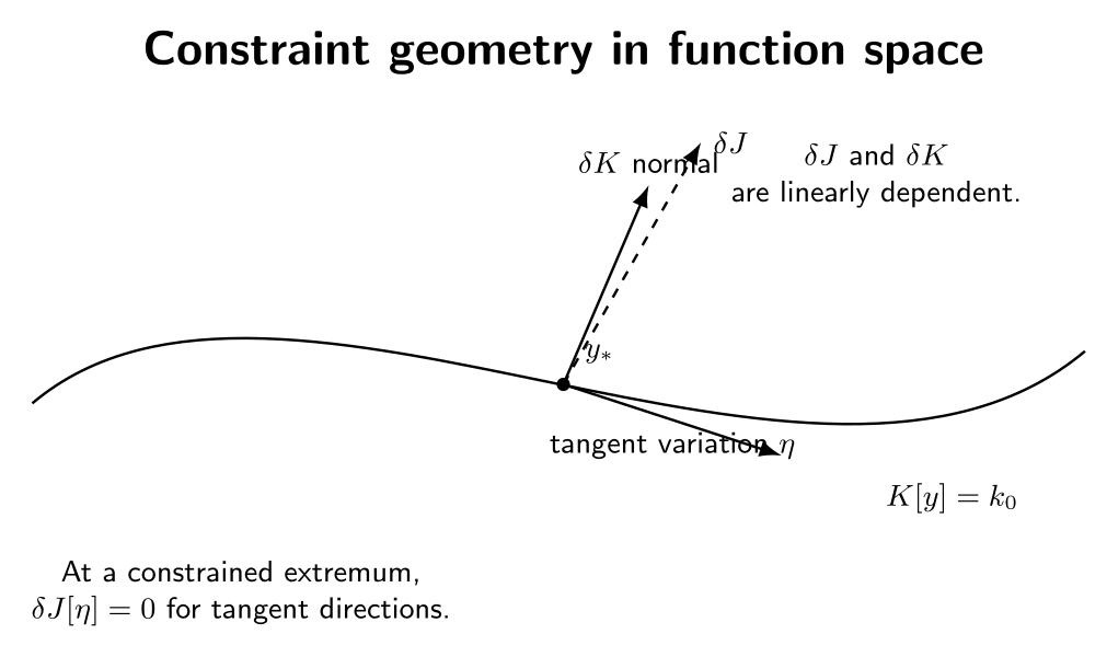
Figure. A constrained extremum is taken over the level set ![K [y] = k0](https://images.physicslibrary.org/cache/objects/1207/make4ht/CalculusOfVariationsConstrainedVariationsAndIsoperimetricProblems10x.png) , not over the
whole function space. At the extremum, admissible first-order variations are tangent to the
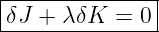
constraint set. The multiplier theorem says that the first variations of
, not over the
whole function space. At the extremum, admissible first-order variations are tangent to the
constraint set. The multiplier theorem says that the first variations of  and
and  are
linearly dependent there.
are
linearly dependent there.
2 Finite-dimensional analogy
For a function  constrained by
an ordinary constrained extremum satisfies
provided  . The geometric reason is that
  is normal to the constraint surface while
the directional derivative of
is normal to the constraint surface while
the directional derivative of  vanishes in every tangent direction. Hence
  must also be
normal to the surface and therefore parallel to
must also be
normal to the surface and therefore parallel to  .
.
In the calculus of variations, the gradients are replaced by first-variation functionals. The
corresponding statement is
The important point is that the multiplier restores the freedom to test against arbitrary
endpoint-preserving directions.
3 The classical one-constraint multiplier theorem
Theorem. Let
with  and
and  sufficiently smooth. Let
 ![y∗ ∈ C2([a,b])](https://images.physicslibrary.org/cache/objects/1207/make4ht/CalculusOfVariationsConstrainedVariationsAndIsoperimetricProblems25x.png) satisfy fixed endpoint conditions and
the constraint
satisfy fixed endpoint conditions and
the constraint ![K [y∗] = k0](https://images.physicslibrary.org/cache/objects/1207/make4ht/CalculusOfVariationsConstrainedVariationsAndIsoperimetricProblems26x.png) . Suppose
. Suppose  is a local constrained extremum of
  . Assume the
constraint is normal at
. Assume the
constraint is normal at  : there exists at least one endpoint-preserving variation
  such
that
such
that
Then there exists a constant  such that
for every endpoint-preserving variation  .
.
3.1 Proof by a two-parameter variation
Take any endpoint-preserving test function  , and use the special direction
  from the
normality assumption. Form
from the
normality assumption. Form
Define two ordinary functions of the two scalar parameters:
and
At the origin,
Moreover,
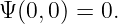
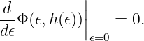
The implicit-function theorem therefore gives, locally, a function  such that
Thus
is a one-parameter family that stays on the constraint surface.
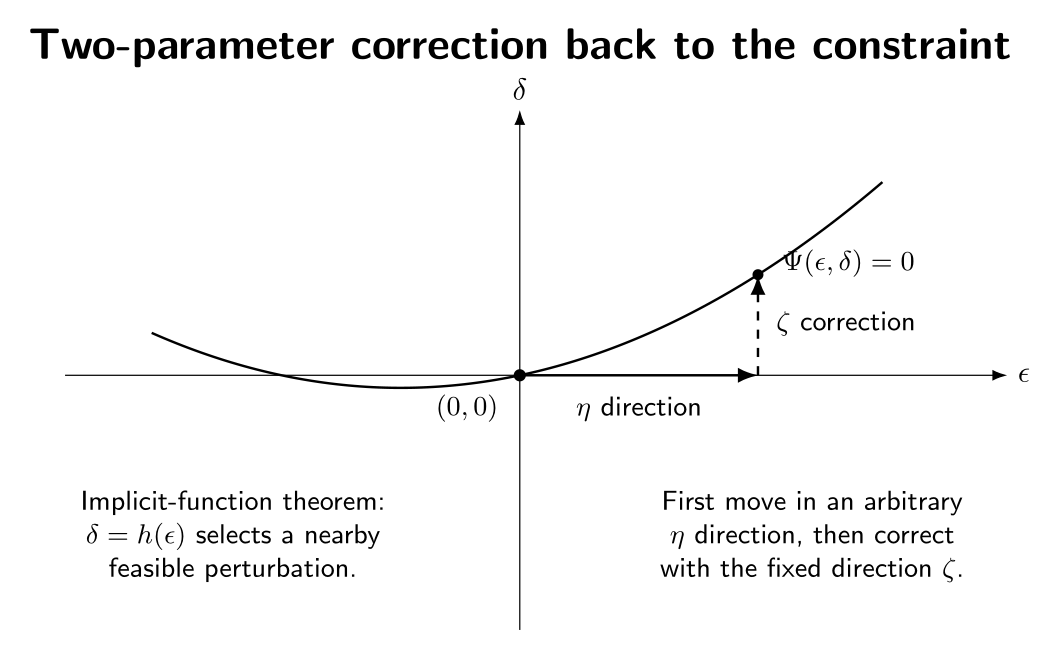
Figure. The two-parameter family supplies one arbitrary direction  and one correction
direction
and one correction
direction  . The constraint equation determines a small correction
  , producing
a feasible curve through parameter space.
, producing
a feasible curve through parameter space.
Because  is a constrained extremum,
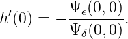
By the ordinary chain rule,
Differentiating the constraint relation gives
so
Substitution yields
Recognize the parameter derivatives as first variations:
and
Define the constant
Then
for every endpoint-preserving  . This proves the theorem. □
4 From the multiplier theorem to Euler–Lagrange
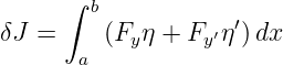
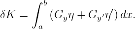
The first variations are
and
Therefore
Introduce the augmented integrand
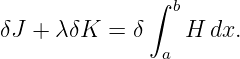
Then
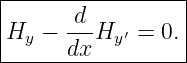
Thus the constrained extremal must satisfy the ordinary Euler–Lagrange equation for
 :
:
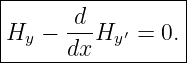
Equivalently,
The original integral constraint must still be imposed after solving this differential equation. It is
normally used to determine the multiplier  or another remaining constant.
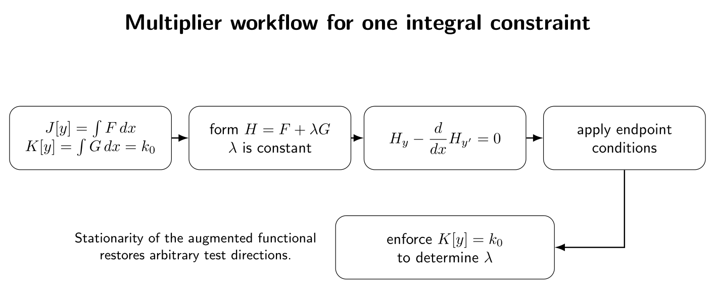
Figure. For a normal integral constraint, augment the integrand by a constant multiplier,
derive the Euler–Lagrange equation for the augmented integrand, apply the endpoint
conditions, and finally enforce the original integral constraint.
5 Why the multiplier is a constant
The condition
is one scalar equation on the entire function. Its multiplier is therefore one scalar constant
 .
.
This should be distinguished from a pointwise constraint such as
A pointwise constraint represents infinitely many scalar conditions, one at each  , and its
multiplier is generally a function
, and its
multiplier is generally a function  . That more mechanical constraint structure will be
developed later in the series.
. That more mechanical constraint structure will be
developed later in the series.
6 Worked example: minimum gradient energy with prescribed mean
Consider
with fixed endpoints
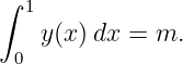
and the integral constraint
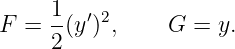
Here
The augmented integrand is
Its derivatives are
The Euler–Lagrange equation is
or
Integrating twice gives
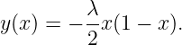
The endpoint conditions imply
so
Now impose the integral constraint:
| m | = − ∫
01x(1 − x) dx ∫
01x(1 − x) dx | (50)
|
| = −  . . | (51) |
Therefore
and
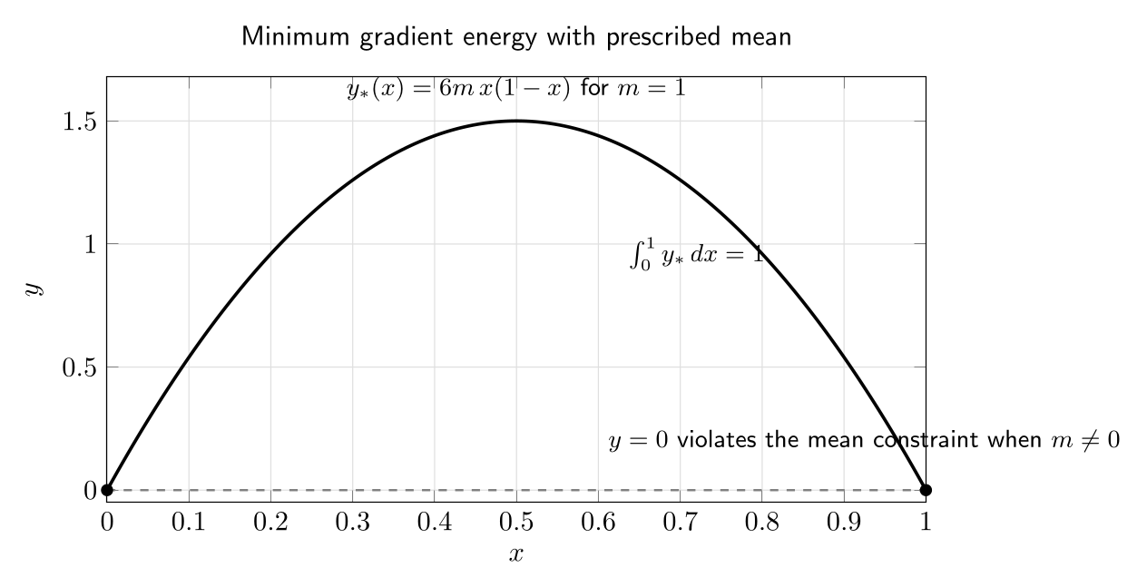
Figure. The fixed-mean constraint forces the minimum-gradient-energy curve away from
the zero function. The stationary curve is a parabola whose amplitude is set by the
prescribed integral  .
.
This example can be classified directly. Let
where
Then
| J[y] | =  ∫
01(y
∗′ + u′)2dx ∫
01(y
∗′ + u′)2dx | (56)
|
| = J[y∗] + ∫
01y
∗′u′dx +  ∫
01(u′)2dx. ∫
01(u′)2dx. | (57) |
Integrating the cross term by parts,
Hence
Equality requires  , and the endpoint conditions then force
  . Thus
  is the
unique global minimizer, not merely a stationary function.
is the
unique global minimizer, not merely a stationary function.
7 Worked example: normalization constraint and an eigenvalue problem
Consider
with
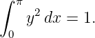
and normalization
Use
Then
so Euler–Lagrange gives
Nontrivial solutions satisfying both endpoint conditions require
with
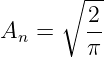
Normalization gives
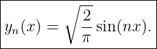
up to an overall sign. Thus
For these stationary functions,
Therefore the lowest branch is
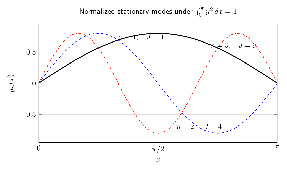
Figure. The normalization constraint converts the multiplier into an eigenvalue parameter.
The stationary functions form discrete sine modes, and the lowest mode has the smallest
gradient energy. This is the elementary variational structure behind later Rayleigh–Ritz
and Sturm–Liouville theory.
The sign assigned to the multiplier is conventional. If the augmented functional is written
 rather than
  , then
  is positive.
8 The classical isoperimetric geometry preview
The name isoperimetric comes from geometric problems in which one quantity, historically
perimeter or length, is fixed while another quantity such as enclosed area is extremized. A graph
version illustrates the multiplier method without yet proving the full closed-curve isoperimetric
theorem.
Suppose one seeks a stationary graph for the area functional
subject to fixed arc length
The augmented integrand is
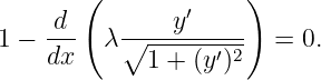
Euler–Lagrange gives
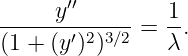
Since  is constant,
The left-hand side is the signed curvature of the graph. Therefore every normal stationary arc has
constant curvature. A nonzero constant-curvature plane curve is a circular arc. The full
isoperimetric theorem requires additional global arguments; CV09E1 will work through the
classical geometry in more detail.
9 Multiple integral constraints
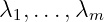
Suppose there are  scalar constraints
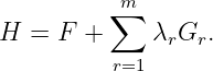
Under the appropriate independence condition, introduce constants
and form
Then a normal constrained extremal satisfies
along with all original constraints and endpoint conditions.
The multiplier vector is determined together with the integration constants. Linear
dependence among the first variations of the constraints requires special care because the
effective number of independent constraints may be smaller than the number written
down.
10 Normal and abnormal extremals
The theorem above assumed that the first variation of the constraint is not the zero functional.
This is the normal case.
If
for every admissible  , then the constraint itself is stationary at
  . The proof based on solving
the constraint for a correction parameter breaks down because the required derivative
. The proof based on solving
the constraint for a correction parameter breaks down because the required derivative  vanishes.
A more general multiplier statement introduces two constants  and
and  , not both zero, such
that
, not both zero, such
that
If  , rescaling gives the normal form used throughout this article. If
  , the extremal
is called abnormal. Abnormality is important in advanced variational theory and optimal
control, but most elementary isoperimetric examples are normal. See [1, 2] for broader
formulations.
, the extremal
is called abnormal. Abnormality is important in advanced variational theory and optimal
control, but most elementary isoperimetric examples are normal. See [1, 2] for broader
formulations.
11 What the multiplier means
The multiplier has several useful interpretations.
First, it is the coefficient that converts the constrained stationarity problem into unconstrained
stationarity of an augmented functional.
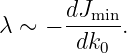
Second, in regular optimization problems it measures the first-order sensitivity of the optimal value
to the prescribed constraint value. Schematically, if
then, subject to sign convention and regularity,
This is the infinite-dimensional analogue of the shadow price interpretation of an ordinary
Lagrange multiplier.
Third, in eigenvalue problems the multiplier often becomes the spectral parameter. The
normalization constraint prevents the trivial zero function, and stationarity selects discrete
eigenfunctions and eigenvalues.
12 Common mistakes
- Varying freely while ignoring the constraint. An arbitrary perturbation normally
leaves the constraint surface.
- Requiring
 for every test function and then applying the
Fundamental Lemma directly. Only tangent directions satisfy the linearized
constraint; the multiplier theorem restores arbitrary test directions through the
augmented functional.
for every test function and then applying the
Fundamental Lemma directly. Only tangent directions satisfy the linearized
constraint; the multiplier theorem restores arbitrary test directions through the
augmented functional.
- Forgetting to impose the original constraint after solving Euler–Lagrange.
The augmented differential equation alone does not determine the multiplier.
- Treating
 as a function of
  for a single scalar integral constraint. The
multiplier is a constant because the constraint is one scalar equation.
for a single scalar integral constraint. The
multiplier is a constant because the constraint is one scalar equation.
- Confusing an integral constraint with a pointwise constraint. Pointwise
constraints generally require multiplier functions.
- Assuming the multiplier condition proves a minimum. It gives a necessary
stationarity condition in the normal case. Classification still requires additional
arguments.
- Forgetting multiplier sign conventions. Writing
 or
or  is
equivalent after redefining the multiplier.
is
equivalent after redefining the multiplier.
- Ignoring abnormal extremals. The simple theorem requires a nondegenerate
constraint first variation.
13 A compact workflow
For one scalar integral constraint, use the following sequence:
- Write the objective functional
![J[y]](https://images.physicslibrary.org/cache/objects/1207/make4ht/CalculusOfVariationsConstrainedVariationsAndIsoperimetricProblems141x.png) .
.
- Write the constraint functional
![K [y] = k0](https://images.physicslibrary.org/cache/objects/1207/make4ht/CalculusOfVariationsConstrainedVariationsAndIsoperimetricProblems142x.png) .
.
- Verify the endpoint conditions and identify admissible variations.
- Check that the constraint is normal, at least at the classical level.
- Introduce a constant multiplier
 .
.
- Form the augmented integrand
 .
.
- Apply the ordinary Euler–Lagrange equation to
 .
.
- Apply all endpoint conditions.
- Impose the original integral constraint to determine
 and remaining constants.
- Separately decide whether the stationary function is a minimum, maximum, or saddle.
14 What CV10 adds
CV09 keeps each extremal smooth across the whole interval but restricts which functions are
admissible through integral constraints. CV10 changes a different assumption: the stationary path
may be only piecewise smooth and may contain an interior corner whose location can
move.
That leads to the Weierstrass–Erdmann corner conditions, which determine which generalized
momentum and Hamiltonian-like quantities must remain continuous across a movable
corner.
Summary
For
subject to the scalar integral constraint
a normal constrained extremal satisfies
for some constant  . Equivalently, with
the extremal satisfies
The multiplier theorem is not merely an algebraic trick. It is the statement that, at a constrained
extremum, the first variation of the objective is linearly dependent on the first variation of the
constraint. This idea reappears in isoperimetric geometry, eigenvalue theory, constrained
mechanics, field theory, and optimal control.
References
[1] I. M. Gelfand and S. V. Fomin, Calculus of Variations, Dover Publications, 2000.
[2] Bruce van Brunt, The Calculus of Variations, Springer, 2004.
[3] Hans Sagan, Introduction to the Calculus of Variations, Dover Publications, 1992.
[4] Gilbert Ames Bliss, Lectures on the Calculus of Variations, University of Chicago
Press, 1946.
[5] Richard Courant and David Hilbert, Methods of Mathematical Physics, Volume I,
Wiley-Interscience, 1989 reprint.

![∫ b
J [y] = F(x,y, y′) dx
a](https://images.physicslibrary.org/cache/objects/1207/make4ht/CalculusOfVariationsConstrainedVariationsAndIsoperimetricProblems0x.png)
![∫ b
K [y] = G (x,y,y ′)dx = k0
a](https://images.physicslibrary.org/cache/objects/1207/make4ht/CalculusOfVariationsConstrainedVariationsAndIsoperimetricProblems1x.png)

![K [y] = k0.](https://images.physicslibrary.org/cache/objects/1207/make4ht/CalculusOfVariationsConstrainedVariationsAndIsoperimetricProblems4x.png)

![K [y𝜖] = K [y] + 𝜖 δK [y;η ] + o(𝜖).](https://images.physicslibrary.org/cache/objects/1207/make4ht/CalculusOfVariationsConstrainedVariationsAndIsoperimetricProblems6x.png)
![δK [y;η] = 0.](https://images.physicslibrary.org/cache/objects/1207/make4ht/CalculusOfVariationsConstrainedVariationsAndIsoperimetricProblems8x.png)


![|----------------------------------------------------------------------|
|δJ[y∗;η] + λδK [y∗;η] = 0 for every admissible endpoint -preserving η.|
-----------------------------------------------------------------------](https://images.physicslibrary.org/cache/objects/1207/make4ht/CalculusOfVariationsConstrainedVariationsAndIsoperimetricProblems21x.png)
![∫ b ∫ b
J [y] = F (x, y,y′)dx, K [y ] = G(x, y,y′) dx,
a a](https://images.physicslibrary.org/cache/objects/1207/make4ht/CalculusOfVariationsConstrainedVariationsAndIsoperimetricProblems22x.png)
![δK [y∗;ζ] ⁄= 0.](https://images.physicslibrary.org/cache/objects/1207/make4ht/CalculusOfVariationsConstrainedVariationsAndIsoperimetricProblems31x.png)
![δJ [y∗;η] + λδK [y∗;η] = 0](https://images.physicslibrary.org/cache/objects/1207/make4ht/CalculusOfVariationsConstrainedVariationsAndIsoperimetricProblems33x.png)

![Φ(𝜖,δ) = J [y𝜖,δ],](https://images.physicslibrary.org/cache/objects/1207/make4ht/CalculusOfVariationsConstrainedVariationsAndIsoperimetricProblems38x.png)
![Ψ (𝜖,δ ) = K [y ] − k .
𝜖,δ 0](https://images.physicslibrary.org/cache/objects/1207/make4ht/CalculusOfVariationsConstrainedVariationsAndIsoperimetricProblems39x.png)
![Ψδ(0,0) = δK [y∗;ζ] ⁄= 0.](https://images.physicslibrary.org/cache/objects/1207/make4ht/CalculusOfVariationsConstrainedVariationsAndIsoperimetricProblems41x.png)





![Φ 𝜖(0, 0) = δJ[y∗;η], Φ δ(0,0 ) = δJ [y∗;ζ],](https://images.physicslibrary.org/cache/objects/1207/make4ht/CalculusOfVariationsConstrainedVariationsAndIsoperimetricProblems54x.png)
![Ψ 𝜖(0,0) = δK [y∗;η], Ψ δ(0, 0) = δK [y∗;ζ ].](https://images.physicslibrary.org/cache/objects/1207/make4ht/CalculusOfVariationsConstrainedVariationsAndIsoperimetricProblems55x.png)
![δJ-[y∗;ζ]
λ = − δK [y∗;ζ].](https://images.physicslibrary.org/cache/objects/1207/make4ht/CalculusOfVariationsConstrainedVariationsAndIsoperimetricProblems56x.png)
![|--------------------------|
|δJ [y ;η] + λδK [y ;η] = 0 |
-----∗------------∗--------](https://images.physicslibrary.org/cache/objects/1207/make4ht/CalculusOfVariationsConstrainedVariationsAndIsoperimetricProblems57x.png)
![∫ b
δJ + λδK = [(Fy + λGy )η + (Fy ′ + λGy ′)η′]dx.
a](https://images.physicslibrary.org/cache/objects/1207/make4ht/CalculusOfVariationsConstrainedVariationsAndIsoperimetricProblems61x.png)


![K [y] = k0](https://images.physicslibrary.org/cache/objects/1207/make4ht/CalculusOfVariationsConstrainedVariationsAndIsoperimetricProblems68x.png)

![∫ 1
J[y] = 1- (y′)2 dx
2 0](https://images.physicslibrary.org/cache/objects/1207/make4ht/CalculusOfVariationsConstrainedVariationsAndIsoperimetricProblems73x.png)








![|----------------∫---------------|
| 1- 1 ′2 |
|J[y] − J[y∗] = 2 (u ) dx ≥ 0. |
-------------------0-------------](https://images.physicslibrary.org/cache/objects/1207/make4ht/CalculusOfVariationsConstrainedVariationsAndIsoperimetricProblems95x.png)
![∫ π
J[y] = (y′)2dx
0](https://images.physicslibrary.org/cache/objects/1207/make4ht/CalculusOfVariationsConstrainedVariationsAndIsoperimetricProblems99x.png)






![2
J [yn] = n .](https://images.physicslibrary.org/cache/objects/1207/make4ht/CalculusOfVariationsConstrainedVariationsAndIsoperimetricProblems109x.png)
![|--------∘-----------------------|
| 2- |
|y1(x) = π sinx, J [y1] = 1.|
----------------------------------](https://images.physicslibrary.org/cache/objects/1207/make4ht/CalculusOfVariationsConstrainedVariationsAndIsoperimetricProblems110x.png)
![∫
b
A [y] = ydx
a](https://images.physicslibrary.org/cache/objects/1207/make4ht/CalculusOfVariationsConstrainedVariationsAndIsoperimetricProblems114x.png)
![∫ b∘ ---------
L[y] = 1 + (y′)2dx = L .
a 0](https://images.physicslibrary.org/cache/objects/1207/make4ht/CalculusOfVariationsConstrainedVariationsAndIsoperimetricProblems115x.png)

![∫ b
Kr [y] = Gr (x,y,y′)dx = kr, r = 1,...,m.
a](https://images.physicslibrary.org/cache/objects/1207/make4ht/CalculusOfVariationsConstrainedVariationsAndIsoperimetricProblems121x.png)
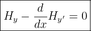
![δK [y∗;η] = 0](https://images.physicslibrary.org/cache/objects/1207/make4ht/CalculusOfVariationsConstrainedVariationsAndIsoperimetricProblems125x.png)


![∫
b ′
J [y] = F(x,y, y) dx
a](https://images.physicslibrary.org/cache/objects/1207/make4ht/CalculusOfVariationsConstrainedVariationsAndIsoperimetricProblems147x.png)
![∫ b
K [y] = G (x,y,y′)dx = k0,
a](https://images.physicslibrary.org/cache/objects/1207/make4ht/CalculusOfVariationsConstrainedVariationsAndIsoperimetricProblems148x.png)