
|
|
|
|||||||
The examples are chosen to make coupling visible. Some systems are coupled through coordinates, some through derivatives, and some become uncoupled only after a change to modal coordinates. The two-mass oscillator provides the central mechanical example because a single scalar action generates the full matrix equation of motion and its normal modes [3, 4, 5].
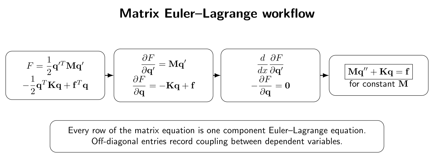
Figure. The matrix Euler–Lagrange workflow for a quadratic vector functional. The matrix notation is compact, but every step represents the same componentwise variational derivatives derived in CV07.
1 How to use this setAttempt the exercises before reading the worked solutions. For each problem, use the following checklist.
Part I: Exercises
Exercise 1: the constant-matrix Euler–Lagrange equationLet
where
Exercise 2: a variable matrix coefficientNow let
with
Exercise 3: derivative coupling and an off-diagonal mass matrixConsider two dependent variables with
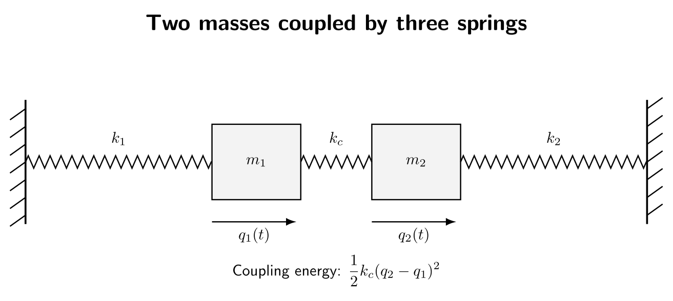
Exercise 4: two masses and three springsTwo masses
Figure. The two-degree-of-freedom oscillator used in Exercises 4–7. The middle spring
stores energy according to the relative displacement
Exercise 5: normal modes of the symmetric two-mass systemSpecialize Exercise 4 to
Seek a normal-mode solution
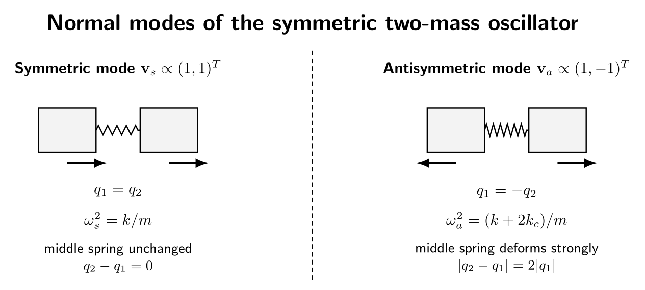
Figure. The two normal-mode shapes of the symmetric oscillator. In the in-phase mode the coupling spring does not change length; in the out-of-phase mode it is stretched or compressed strongly and raises the modal frequency.
Exercise 6: diagonalization with modal coordinatesFor the same symmetric oscillator, define
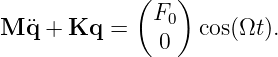
Exercise 7: harmonic forcing in matrix formAdd an applied force to the symmetric two-mass system:
Assume an undamped steady harmonic response
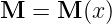
Exercise 8: a coupled boundary-value problemConsider the static variational problem
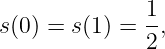
with fixed endpoint data
Figure. A representative stationary solution of the coupled boundary-value problem. The average coordinate remains linear, while the difference coordinate is suppressed in the interior by the coupling penalty.
Part II: Complete worked solutions
Solution 1: the constant-matrix Euler–Lagrange equationWrite
Because
One way to verify this without memorizing a matrix-calculus rule is to write
Differentiating with respect to
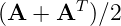
Symmetry Similarly,
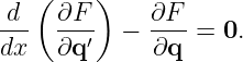
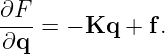
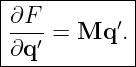
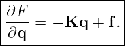
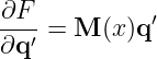
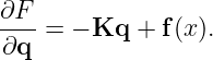
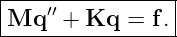
The vector Euler–Lagrange equation is
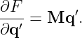
Since
For
This is the matrix version of the scalar linear Euler–Lagrange equation. The matrix form is compact, but no new variational principle was introduced; it is just the collection of all component equations.
Solution 2: a variable matrix coefficientNow
and
Therefore the Euler–Lagrange equation is naturally written as
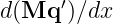
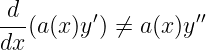
This divergence form is often the safest form because it preserves the exact result of integration by parts. Expanding with the matrix product rule,
Thus
The term
when
Solution 3: derivative coupling and an off-diagonal mass matrixThe integrand is
For
Therefore
Likewise,
Define
Then
The eigenvalues of
A real symmetric matrix is positive definite exactly when all its eigenvalues are positive. Therefore
which combine to give
Thus derivative coupling appears as an off-diagonal entry in the matrix multiplying the highest derivative. In mechanics that matrix is often the mass matrix.
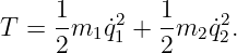
Solution 4: two masses and three springsThe kinetic energy is
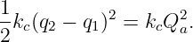
The three spring energies are
Hence
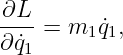
For
and
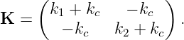
Thus
For
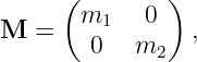
Define
and
Then
The off-diagonal terms
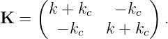
Solution 5: normal modes of the symmetric two-mass systemFor
and
Insert
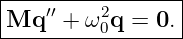
Since
the equation of motion becomes
A nonzero mode shape exists only if
Therefore
The determinant gives
Factoring,
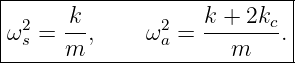
Thus
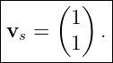
For
so one mode vector is
For
so
The physical interpretation is especially useful. In the symmetric mode,
so the coupling spring is neither stretched nor compressed. It contributes no restoring force and therefore does not change the frequency. In the antisymmetric mode,
so the coupling spring deforms strongly, increasing the restoring stiffness and raising the frequency [5, 6].
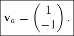
Solution 6: diagonalization with modal coordinatesThe coordinate transformation is
Solving for the original coordinates,
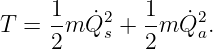
The same relations hold for the velocities. Therefore
Hence
For the wall springs,
The coupling displacement is
so
Therefore
The Lagrangian becomes
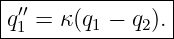
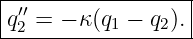
The two coordinates are now uncoupled. Their equations are
and
which immediately reproduce
This is the simplest example of modal diagonalization: a coupled coordinate system becomes two independent oscillators after changing basis to eigenvector coordinates.
Solution 7: harmonic forcing in matrix formThe forced equation is
Assume
Then
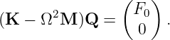
so cancellation of the common cosine factor yields
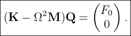
For the symmetric system, define
Then
The determinant is
Away from
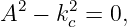
The undamped response becomes singular when
which factors exactly as in Exercise 5:
Thus resonance occurs at
This is not a new variational condition. The variational principle generated the matrix differential equation; ordinary linear-system analysis then reveals its resonant response.
Solution 8: a coupled boundary-value problemThe integrand is
For
Therefore
For
so
Introduce
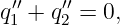
Adding the two differential equations gives
hence
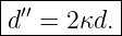
Subtracting them gives
so
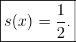
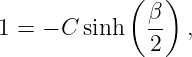
The boundary data imply
so
For the difference,
Let
The antisymmetry of the boundary data about
Using
so
Finally,
which gives
and
Increasing
2 What these problems should teachThe most useful habit is to separate three layers of the calculation.
Confusing these layers can make the matrix notation look more mysterious than it is. The matrices do not replace the variational derivation; they organize its result.
3 Common mistakes
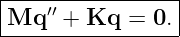
SummaryFor a quadratic vector functional with constant symmetric matrices,
the vector Euler–Lagrange equations reduce to
In mechanics,
For the symmetric two-mass oscillator, the coupled coordinate equations have normal modes
with
The modal coordinates diagonalize the same scalar action that originally produced the coupled equations. CV07E2 next applies vector variational methods to trajectory and geometry problems, while CV08 extends the theory to functionals involving higher derivatives.
References
[1] I. M. Gelfand and S. V. Fomin, Calculus of Variations, Dover Publications, 2000. [2] Bruce van Brunt, The Calculus of Variations, Springer, 2004. [3] Cornelius Lanczos, The Variational Principles of Mechanics, 4th ed., Dover Publications, 1986. [4] Herbert Goldstein, Charles Poole, and John Safko, Classical Mechanics, 3rd ed., Addison Wesley, 2002. [5] Leonard Meirovitch, Elements of Vibration Analysis, 2nd ed., McGraw-Hill, 1986. [6] S. S. Rao, Mechanical Vibrations, 5th ed., Prentice Hall, 2011. "Calculus of Variations: Coupled Systems and Matrix Euler--Lagrange Equations" is owned by bloftin.
This object's parent. Cross-references: CV08, CV07E2, boundary, differential equation, coordinate system, velocities, determinant, mechanics, matrix product, variational principle, static, algebraic, resonance, amplitude, force, relations, frequencies, energy, Lagrange equations, potential energy, kinetic energy, equilibrium, displacements, masses, divergence, symmetric matrices, dimensions, Lagrangian, vector, normal modes, matrix, oscillator, system, scalar, CV07 There are 2 references to this object. This is version 1 of Calculus of Variations: Coupled Systems and Matrix Euler--Lagrange Equations, born on 2026-10-11. Object id is 1470, canonical name is CalculusOfVariationsCoupledSystemsAndMatrixEulerLagrangeEquations. Accessed 3 times total. Classification:
|
|
|
|
Pending Errata and AddendaNone.
|
DiscussionNo messages.
|
Interact |
![[parent]](https://images.physicslibrary.org/images/uparrow.png)
 . This
companion article develops the computational side of that extension. The main objective is to
become comfortable moving among three equivalent descriptions of the same stationary
. This
companion article develops the computational side of that extension. The main objective is to
become comfortable moving among three equivalent descriptions of the same stationary

 .
.
 or
or  .
.
 and
and  component by component if there is any doubt about
the matrix derivative.
component by component if there is any doubt about
the matrix derivative.
 or an equivalent sinusoidal
ansatz.
or an equivalent sinusoidal
ansatz.
 and consider
![∫ [ ]
b 1-′T ′ 1- T T
J[q] = 2q Mq − 2 q Kq + f q dx,
a](https://images.physicslibrary.org/cache/objects/1470/make4ht/CalculusOfVariationsCoupledSystemsAndMatrixEulerLagrangeEquations10x.png)
 and
and  are constant
  is a constant vector.
 .
.![∫ b[ ]
J[q] = 1q′TM (x)q ′ − 1-qTKq + f(x )T q dx,
a 2 2](https://images.physicslibrary.org/cache/objects/1470/make4ht/CalculusOfVariationsCoupledSystemsAndMatrixEulerLagrangeEquations17x.png)
 .
.
 by
by  is generally incorrect.
![∫ b[ ]
J[q1,q2] = 1q ′2+ αq′q′+ 1q′2− 1ω2(q2 + q2) dx.
a 2 1 1 2 2 2 2 0 1 2](https://images.physicslibrary.org/cache/objects/1470/make4ht/CalculusOfVariationsCoupledSystemsAndMatrixEulerLagrangeEquations21x.png)

 .
.
 makes the derivative quadratic form positive
definite.
makes the derivative quadratic form positive
definite. and
and  move horizontally. Mass 1 is attached to the left wall by spring
  ,
mass 2 is attached to the right wall by spring
,
mass 2 is attached to the right wall by spring  , and the masses are connected by spring
  .
Let
.
Let  and
and  be
be  .
.
 .
.
 .
.

 and
and  .
.
 , which is the source of
coordinate coupling.
, which is the source of
coordinate coupling.




 in terms of
  .
.
 and
and  directly from the separated Lagrangian.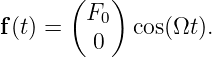

 and
and  away from
  at which the undamped
 ![∫ 1[1 1 κ ]
J[q1,q2] = --q′21 + --q′22 + -(q1 − q2)2 dx, κ > 0,
0 2 2 2](https://images.physicslibrary.org/cache/objects/1470/make4ht/CalculusOfVariationsCoupledSystemsAndMatrixEulerLagrangeEquations54x.png)


 and
and  .
.
 and
and  .
.
 does to the two profiles.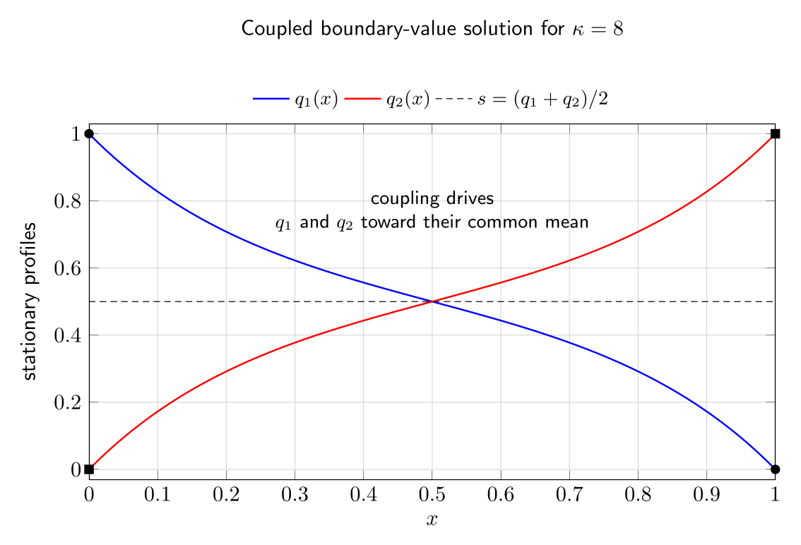

 is symmetric, differentiating the quadratic form with respect to
  gives
gives
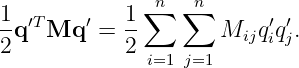
 produces
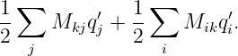
 makes the two sums equal, giving the
  -th component of
 .
.

 is constant,
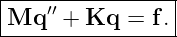
 ,
,
![|-----------------------------|
|d--[M (x )q′(x )] + Kq = f(x). |
-dx---------------------------|](https://images.physicslibrary.org/cache/objects/1470/make4ht/CalculusOfVariationsCoupledSystemsAndMatrixEulerLagrangeEquations80x.png)


 disappears only when
  is constant. This is the matrix analogue of the scalar
warning
is constant. This is the matrix analogue of the scalar
warning
 .
.

 ,
,




 are
are





 ,
,


![[ ]
1 2
2kc(q2 − q1)](https://images.physicslibrary.org/cache/objects/1470/make4ht/CalculusOfVariationsCoupledSystemsAndMatrixEulerLagrangeEquations105x.png)

 ,
,


 encode the fact that the middle spring depends on relative
displacement. The matrix is symmetric because the spring stores a scalar potential energy and the
mixed second derivatives agree.
encode the fact that the middle spring depends on relative
displacement. The matrix is symmetric because the spring stores a scalar potential energy and the
mixed second derivatives agree.
 and
and  ,
,







![[k − m ω2 ][k + 2k − m ω2] = 0.
c](https://images.physicslibrary.org/cache/objects/1470/make4ht/CalculusOfVariationsCoupledSystemsAndMatrixEulerLagrangeEquations123x.png)
 , the matrix equation gives

 ,
,









![|----[---------------]---[----------------------]--|
|L = 1m Q˙2 − 1kQ2 + 1-m ˙Q2 − 1-(k + 2kc)Q2 .|
| 2 s 2 s 2 a 2 a |
----------------------------------------------------](https://images.physicslibrary.org/cache/objects/1470/make4ht/CalculusOfVariationsCoupledSystemsAndMatrixEulerLagrangeEquations141x.png)








 , the inverse matrix gives

![[k − m Ω2 ][k + 2kc − m Ω2] = 0.](https://images.physicslibrary.org/cache/objects/1470/make4ht/CalculusOfVariationsCoupledSystemsAndMatrixEulerLagrangeEquations155x.png)


 ,
,

 ,
,






 suggests the centered form
![[ ( 1 )]
d(x) = C sinh β x − -- .
2](https://images.physicslibrary.org/cache/objects/1470/make4ht/CalculusOfVariationsCoupledSystemsAndMatrixEulerLagrangeEquations174x.png)
 ,
,
![|-------------[--(------)]-|
| sinh β x − 1 |
|d(x) = − ------------2---.|
-------------sinh(β∕2-)----|](https://images.physicslibrary.org/cache/objects/1470/make4ht/CalculusOfVariationsCoupledSystemsAndMatrixEulerLagrangeEquations177x.png)

![|------------------[--(-----)]-|
| 1- 1-sinh--β--x-−-12---|
|q1(x ) = 2 − 2 sinh (β∕2) |
--------------------------------](https://images.physicslibrary.org/cache/objects/1470/make4ht/CalculusOfVariationsCoupledSystemsAndMatrixEulerLagrangeEquations179x.png)
![|------------------[--(-----)]-|
| 1 1sinh β x − 12 |
q2(x) = 2 + 2----sinh-(β-∕2)---.|
--------------------------------](https://images.physicslibrary.org/cache/objects/1470/make4ht/CalculusOfVariationsCoupledSystemsAndMatrixEulerLagrangeEquations180x.png)
 increases
  . The functional penalizes differences between
  and
and
 more strongly, so the two stationary profiles are pulled closer to their common
mean
more strongly, so the two stationary profiles are pulled closer to their common
mean  through most of the interior while still satisfying their opposing endpoint
values.
through most of the interior while still satisfying their opposing endpoint
values.

 , the derivative of
  involves the symmetric part
 .
.
 , then
 .
.
 , while the final equation is normally
  .
.
![∫ [1 1 ]
J[q] = -q ′T Mq ′ − -qT Kq + fTq dx,
2 2](https://images.physicslibrary.org/cache/objects/1470/make4ht/CalculusOfVariationsCoupledSystemsAndMatrixEulerLagrangeEquations194x.png)
 becomes time and the same structure gives


