Strapdown Inertial Navigation: Earth Rotation and Navigation Frames
A strapdown inertial navigation system does not evolve one vector in one coordinate system. It
continually moves information among several frames that rotate with respect to one another. The
gyroscopes measure body angular rate relative to inertial space. Position is usually reported
relative to the rotating Earth. Velocity is often represented in a local north-east-down frame.
Accelerometer specific force begins in body axes and must be rotated into the chosen navigation
frame before it can be integrated.
The purpose of this entry is to make those frames and their relative angular rates explicit. The key
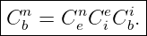
chain is
where i denotes an Earth-centered inertial frame, e an Earth-centered Earth-fixed frame, n a local
north-east-down navigation frame, and b the vehicle body frame. The corresponding relative
angular rates are
The first is Earth rotation. The second is the transport rate, caused by motion over Earth’s curved
surface. The third is the vehicle’s rotation relative to the local navigation frame. Their combination
determines the rate that must be removed from the inertial gyro measurement before the body
attitude relative to NED can be propagated [1, 2, 3].
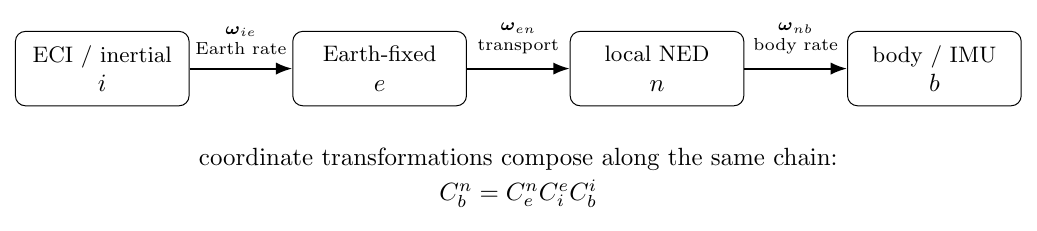
Figure. The principal reference frames used in a local-level strapdown mechanization.
Each neighboring frame rotates relative to the previous one, and coordinate
transformations compose along the same chain.
1 Learning objectives
After completing this entry, the reader should be able to:
- distinguish ECI, ECEF, local NED, and body frames physically and mathematically;
- interpret the notation ωabc as the angular velocity of frame b relative to frame a,
resolved in frame c;
- write the ECI-to-ECEF coordinate transformation and its time derivative;
- derive the ECEF-to-NED direction cosine matrix from the local north, east, and down
basis vectors;
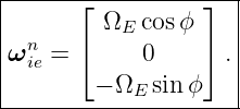
- derive Earth rate resolved in NED;
- derive the WGS-84 meridian and prime-vertical radii of curvature used in local position
kinematics;
- derive the geodetic rates dϕ∕dt, dλ∕dt, and dh∕dt from NED velocity;
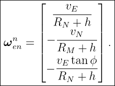
- derive the NED transport-rate vector ωenn;
- form the total navigation-frame inertial rate ωinn;
- convert inertial gyro measurements ωibb into body rate relative to NED;
- derive the strapdown attitude equation from frame-rate composition;
- show how the ECEF velocity equation transforms into the NED velocity equation;
- identify coordinate singularities and frame-selection issues near the poles;
- construct numerical checks that detect frame-order and sign errors in navigation
software.
2 Frame notation
Throughout this series, a superscript indicates the frame in which vector components are resolved.
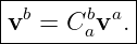
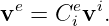
A direction cosine matrix
maps components from frame a into frame b:
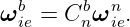
Angular velocity uses two frame subscripts and one resolution superscript. In
the first subscript is the reference frame, the second subscript is the rotating frame, and the
superscript gives the frame in which the vector components are written. Thus
means the angular velocity of the Earth-fixed frame e relative to inertial frame i, resolved in NED
coordinates.
This convention is worth enforcing rigorously. A physical angular-velocity vector is independent of
coordinates, but its numerical components are not. For example,
The vector is the same Earth rotation in both equations. Only the coordinate representation has
changed.
3 The Earth-centered inertial frame
An Earth-centered inertial frame has its origin at Earth’s center of mass, but its axes do not rotate
with the solid Earth. For navigation derivations it is convenient to choose the zi axis
approximately along Earth’s spin axis and to choose the xi and yi axes fixed relative to inertial
space.
No Earth-centered realization is perfectly inertial over arbitrary time scales. Earth’s spin axis
precesses and nutates, and the planet moves around the Sun. For the strapdown derivations in this
series, ECI is the reference frame in which Newton’s second law takes its simplest form.
Higher-fidelity astronomical realizations can be introduced when required.
In an inertial frame the ideal translational equation from INS03 and INS05 has the clean
form
There is no Coriolis term and no centrifugal term because those are consequences of
expressing the dynamics in rotating coordinates. This simplicity makes ECI valuable
conceptually even when the operational navigation solution is maintained in ECEF or
NED.
4 The Earth-centered Earth-fixed frame
The Earth-centered Earth-fixed frame shares the same origin as ECI, but its axes rotate with
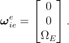
Earth. We use
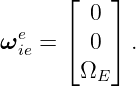
for the angular velocity of ECEF relative to ECI. To first order for the present discussion its
magnitude is the WGS-84 nominal Earth rotation rate
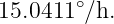
The magnitude corresponds to about
That rate is small compared with typical vehicle body rates, but it is not small compared with
precision inertial sensor biases. It is therefore a first-order navigation quantity.
4.1 A simple ECI-to-ECEF transformation
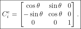
Let 𝜃 be the Earth rotation angle measured about the common z axis. With the passive coordinate
convention of INS01, one convenient idealized transformation is
Therefore
Differentiating the matrix while using d𝜃∕dt = ΩE gives
where
The negative sign is a consequence of the passive transformation. The ECEF axes rotate positively
relative to inertial space, so the components of an inertially fixed vector appear to rotate
oppositely when written in ECEF coordinates.
5 Geodetic position on the WGS-84 ellipsoid
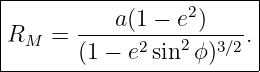
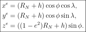
Local navigation frames are attached to a position on a reference ellipsoid. Let
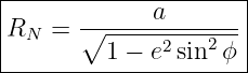
For an ellipsoid with semi-major axis a and eccentricity squared e2, define the prime-vertical radius
of curvature
and the meridian radius of curvature
The geodetic coordinates map to ECEF position through
These equations distinguish geodetic latitude from the geocentric angle discussed in INS05E2. The
local vertical used by a normal-gravity navigation frame is aligned with the ellipsoid Normal, not
generally with the radius vector from Earth’s center.
6 The local north-east-down frame
The NED frame is attached to the vehicle’s local geodetic position. Its axes are
North is tangent to the reference ellipsoid in the direction of increasing geodetic latitude. East is
tangent in the direction of increasing longitude. Down points opposite the ellipsoid outward
normal.
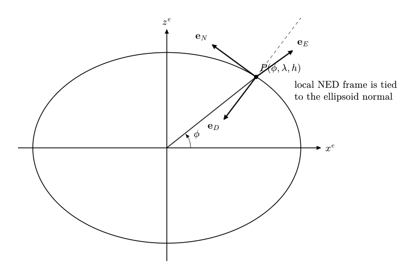
Figure. The NED navigation frame is a local tangent frame tied to the reference ellipsoid.
As the vehicle changes latitude or longitude, the local basis itself rotates even if the vehicle
maintains a fixed heading relative to local level.
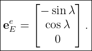
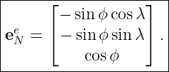
6.1 NED basis vectors expressed in ECEF
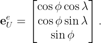
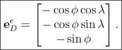
The outward ellipsoid-normal unit vector is
Therefore the down unit vector is
A unit vector tangent to increasing longitude is
The north vector completing the right-handed NED triad is
For NED axes the handedness relation is
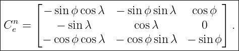
6.2 ECEF-to-NED direction cosine matrix
From INS01, the rows of Cen are the NED basis vectors expressed in ECEF coordinates.
Hence
As always for a proper DCM,
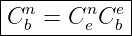
The body-to-NED transformation can therefore be assembled through intermediate frames. For
example,
or, if attitude is first known relative to ECI,
This is a practical expression of the composition rule derived in INS01.
7 Earth rate resolved in NED
Earth rotation is simplest in ECEF coordinates:
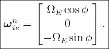
To obtain the same physical vector in NED components,
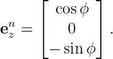
Using the third column of Cen gives
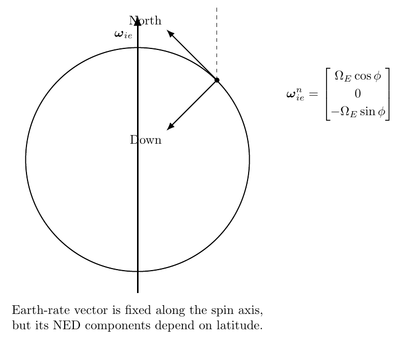
Figure. Earth’s angular-velocity vector is parallel to the spin axis. Resolving that fixed
vector into local NED axes produces a north component ΩE cos ϕ and a down component
−ΩE sin ϕ.
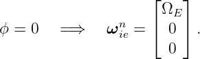
Several immediate checks are useful.
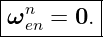
At the equator,
Earth rate points north in local coordinates.
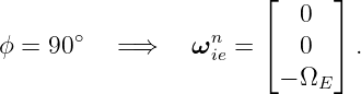
At the North Pole,
Earth rate points upward, which is negative down.
At 45∘ latitude,
These are the same Earth-rate components used in the gyroscope examples of INS04E1.
8 Position kinematics from NED velocity
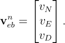
Let local velocity relative to Earth be
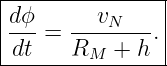
A displacement northward by dsN changes geodetic latitude according to the local meridian radius
of curvature:
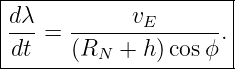
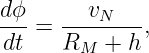
Dividing by time gives
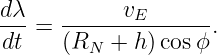
An eastward displacement follows a parallel of latitude whose local radius is (RN + h) cos ϕ.
Therefore
so
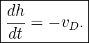
Finally, because the third NED axis points down while ellipsoidal height is positive
upward,
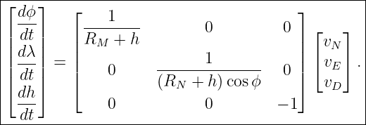
Together,
This is the local-level position mechanization introduced in INS00, now derived from ellipsoid
geometry.
9 Why the local navigation frame rotates
Suppose a vehicle moves north while maintaining zero roll, pitch, and heading relative to local
NED. The vehicle is following Earth’s curved surface. The local down direction at its new location
is not parallel to the local down direction at its old location. Therefore the NED frame has rotated
relative to ECEF even though the vehicle did not deliberately turn relative to local
level.
The same effect occurs during eastward motion. In addition to following a curved parallel, the
directions called north and east change with longitude. This rotation of the local navigation frame
caused by translational motion is the transport rate.
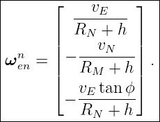
10 Derivation of the NED transport rate
Let
be the angular velocity of the local NED frame relative to ECEF, resolved in NED
coordinates.
There are two geometric contributions.
10.1 Change of latitude
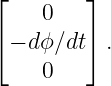
Increasing geodetic latitude rotates the local NED frame about its east axis. With the NED sign
convention, the corresponding angular velocity is
The negative sign can be checked at the equator. Moving north tips the local down vector
toward north, which corresponds to a negative rotation about east under the right-hand
rule.
10.2 Change of longitude
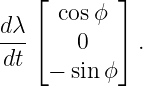
Increasing longitude rotates the local meridian around Earth’s spin axis. The angular velocity
associated with this change is
The Earth spin axis resolved in NED has the same geometry as Earth rate, except without the
factor ΩE:
Therefore the longitude contribution is
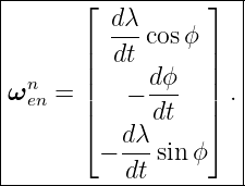
Adding latitude and longitude contributions gives
Now substitute the position-rate equations:
The result is the standard NED transport rate
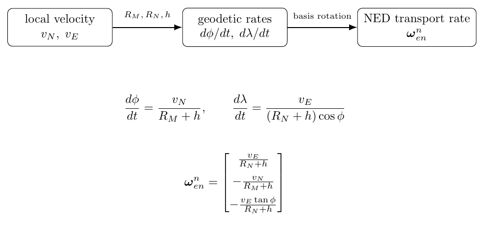
Figure. Local velocity changes geodetic latitude and longitude. Those position rates rotate
the NED basis relative to ECEF, producing the transport rate ωenn.
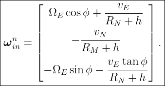
11 Total navigation-frame angular rate relative to inertial space
Angular velocities add when they are expressed in the same coordinates. Since ECEF rotates
relative to ECI and NED rotates relative to ECEF,
Substituting the Earth-rate and transport-rate expressions gives
This vector is one of the most important reference-rate quantities in a local-level strapdown
navigator.
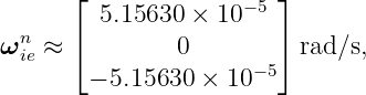
11.1 Numerical scale example
Consider
Using WGS-84,
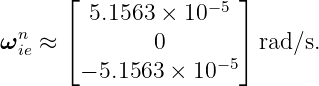
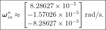
Earth rate is
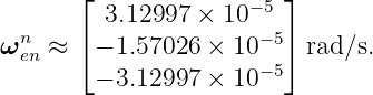
while transport rate is
Therefore
The transport-rate magnitude in this example is about 9.69∘∕h, which is not negligible compared
with Earth’s 15.04∘∕h rotation rate. Fast motion over Earth can therefore make transport rate a
major part of the attitude reference-rate correction.
12 From inertial gyro rate to body rate relative to NED
An ideal strapdown gyro measures
the body frame relative to inertial space, resolved in body coordinates.
But attitude Cbn describes the body relative to the navigation frame. The desired relative angular
velocity is therefore
The angular-rate chain is
All terms must be represented in the same frame before subtraction. Resolving in body
coordinates,
Hence
Using the previous result,
This equation explains why a navigation-grade gyro correction depends on both current position
and current velocity. Latitude determines Earth rate in NED, while velocity and ellipsoid curvature
determine transport rate.
13 Derivation of the strapdown attitude equation
INS04 introduced the result
We can now interpret every term.
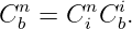
Start with the composition
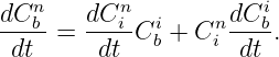
Differentiate:
For the inertial-to-navigation passive transformation,
For body axes rotating relative to inertial space,
Substitution gives
Since CinC
bi = C
bn,
Finally,
The first term advances attitude using the inertial angular rate measured by the gyros. The second
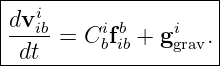
term removes the rotation of the navigation frame itself.
14 ECEF velocity dynamics
INS05 showed that when effective gravity already contains centrifugal acceleration, the ECEF
velocity equation is
This equation contains Earth rate but not transport rate. That is because ECEF is a global
Earth-fixed frame. It rotates with Earth, but it does not rotate further as the vehicle moves across
the surface.
Transport rate appears only after the velocity coordinates are expressed in the moving local NED
frame.
15 Deriving the NED velocity equation from ECEF
Start from
Differentiate:
Because NED rotates relative to ECEF at ωenn,
Thus
Substitute the ECEF equation:
Use
and the cross-product transformation identity from INS01,
Therefore
The transport-rate term has now appeared explicitly because the coordinate frame used for
velocity moves over the ellipsoid with the vehicle.
16 The full local-level mechanization loop
The frame structure developed in this entry closes several feedback loops in the navigation
computation.
Position provides ϕ, λ, and h. These determine the local ECEF-to-NED transformation, Earth-rate
components, curvature radii, and gravity model. Velocity provides vN and vE, which determine
transport rate. Earth rate and transport rate correct the gyro measurements and enter the velocity
equation. Updated attitude rotates accelerometer specific force into NED. Updated velocity then
advances position.

Figure. Frame transformations and reference-frame rates form a coupled loop. Position
and velocity are not merely outputs of the strapdown mechanization. They also determine
the reference-frame corrections needed to propagate the next attitude and velocity state.
A local-level strapdown navigator therefore has the coupled structure
Every quantity in these equations has now been connected either to sensor physics, rotating-frame
kinematics, Earth geometry, or gravity modeling.
17 Body-frame conventions
The body frame b is fixed to the IMU or vehicle. In this series the default convention is
forward-right-down:
This convention is common in aerospace inertial navigation, but not universal. Robotics software
often uses forward-left-up or other conventions. A DCM that is algebraically correct for one
body-axis convention can be physically wrong for another.
A robust implementation should therefore document three items independently:
- the physical direction of each sensor axis;
- the coordinate convention expected by the navigation mechanization;
- the exact DCM or permutation used to map sensor coordinates into the mechanization
body frame.
Axis convention errors often mimic attitude-sign or gravity-sign errors and can be difficult to
isolate after integration begins.
18 Local-level singularity near the poles
The longitude-rate equation contains
As |ϕ|→ 90∘, longitude becomes poorly conditioned because all meridians converge at the pole.
The transport-rate down component also contains
This is not a physical singularity in vehicle motion. It is a coordinate singularity of the
conventional local-level parameterization.
High-latitude systems can avoid the problem by using ECEF mechanization, wander-azimuth
frames, grid navigation frames, or other local coordinate constructions designed to remain well
conditioned near the poles [1, 2].
19 Implementation checks
Frame mathematics is unusually vulnerable to sign, transpose, and ordering mistakes. Several tests
should be built into a strapdown implementation.
19.1 DCM orthogonality
Every proper frame transform should satisfy
19.2 Round-trip transformation
For an arbitrary vector,
should reproduce the original vector to numerical precision.
19.3 Earth-rate limiting cases
At the equator,
At the North Pole,
A code result with the opposite down sign usually indicates either an ENU/NED mismatch or an
incorrect ECEF-to-local DCM.
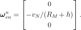
19.4 Zero-velocity transport rate
If
then
A stationary Earth-fixed vehicle still sees Earth rate, but it has no transport rate.
19.5 Pure north motion
If vE = 0,
Only the east-axis transport component remains.
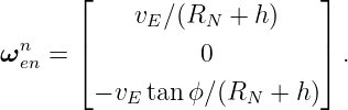
19.6 Pure east motion
If vN = 0,
This makes a useful test of both the north and down transport components.
20 What the IMU knows and what the navigator must know
A useful conceptual distinction is that the IMU alone does not know latitude, longitude, ellipsoid
curvature, or transport rate. The gyroscopes provide ωibb. The accelerometers provide f
ibb. The
navigation computer supplies the Earth and geometry model needed to interpret those inertial
measurements in an Earth-relative frame.
For a local-level mechanization the computer must maintain or compute
This separation is fundamental. The sensors measure inertial quantities. The Earth model supplies
the rotating reference frame in which navigation outputs are desired.
21 Connection to subsequent strapdown lessons
The next articles use the frame structure developed here repeatedly.
INS07 will use
to develop attitude propagation in greater detail.
INS08 will reformulate the same rotational kinematics using quaternions and finite incremental
rotations.
INS09 will use gravity and Earth rate as reference vectors for initial alignment.
INS12 will construct the complete ECEF mechanization, where no local transport-rate correction
appears explicitly.
INS13 and INS14 will return to local-level transport rate and ellipsoidal position kinematics in
greater numerical detail.
INS15 will assemble the full NED attitude, velocity, and position mechanization into one
continuous system.
22 Summary
The essential frame relationships are
Earth rate in NED is
Transport rate is
The local geodetic position rates are
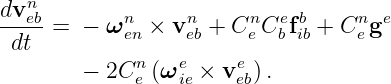
The gyro rate needed for attitude relative to NED is
The corresponding attitude equation is
Finally, the NED velocity equation is
The purpose of the frame hierarchy is now clear. Earth rotation, motion over the ellipsoid, body
motion, gravity, and IMU measurements all refer to different physical relationships. Strapdown
navigation works only when those relationships are transformed into common coordinates with the
correct frame ordering and angular-rate signs.
References
[1] David H. Titterton and John L. Weston, Strapdown Inertial Navigation Technology,
2nd ed., Institution of Electrical Engineers, 2004.
[2] Paul D. Groves, Principles of GNSS, Inertial, and Multisensor Integrated Navigation
Systems, 2nd ed., Artech House, 2013.
[3] Christopher Jekeli, Inertial Navigation Systems with Geodetic Applications, Walter
de Gruyter, 2001.
[4] Paul G. Savage, “Strapdown Inertial Navigation Integration Algorithm Design Part
1: Attitude Algorithms,” Journal of Guidance, Control, and Dynamics, vol. 21, no. 1,
pp. 19–28, 1998.
[5] Paul G. Savage, “Strapdown Inertial Navigation Integration Algorithm Design Part
2: Velocity and Position Algorithms,” Journal of Guidance, Control, and Dynamics, vol.
21, no. 2, pp. 208–221, 1998.
[6] National Geospatial-Intelligence Agency, Department of Defense World Geodetic
System 1984: Its Definition and Relationships with Local Geodetic Systems,
NGA.STND.0036, Version 1.0.0, 2014.








![|---e--------------|
|dC-i= − [ωe ]×Ce ,|
--dt--------ie---i--](https://images.physicslibrary.org/cache/objects/1354/make4ht/StrapdownInertialNavigationEarthRotationAndNavigationFrames13x.png)


















![dCn
---b-= Cnb [ωbib]× − [ωnin]×Cnb .
dt](https://images.physicslibrary.org/cache/objects/1354/make4ht/StrapdownInertialNavigationEarthRotationAndNavigationFrames64x.png)
![dCn
--i-= − [ωnin ]×Cni .
dt](https://images.physicslibrary.org/cache/objects/1354/make4ht/StrapdownInertialNavigationEarthRotationAndNavigationFrames67x.png)
![i
dC-b= Ci[ωb ]×.
dt b ib](https://images.physicslibrary.org/cache/objects/1354/make4ht/StrapdownInertialNavigationEarthRotationAndNavigationFrames68x.png)
![dCnb- n n i n i b
dt = − [ω in]×C i C b + C i C b[ω ib]×.](https://images.physicslibrary.org/cache/objects/1354/make4ht/StrapdownInertialNavigationEarthRotationAndNavigationFrames69x.png)
![|----------------------------|
|dCnb- n b n n |
| dt = C b [ω ib]× − [ω in]×C b .
------------------------------](https://images.physicslibrary.org/cache/objects/1354/make4ht/StrapdownInertialNavigationEarthRotationAndNavigationFrames70x.png)
![|---n------------------------------|
|dCb--= Cn [ωb ] − [ωn + ωn ] Cn .|
--dt------b--ib×------ie----en-×--b--](https://images.physicslibrary.org/cache/objects/1354/make4ht/StrapdownInertialNavigationEarthRotationAndNavigationFrames71x.png)



![n
dC-e-= − [ωn ]×Cn .
dt en e](https://images.physicslibrary.org/cache/objects/1354/make4ht/StrapdownInertialNavigationEarthRotationAndNavigationFrames75x.png)




![|----------------------------------------|
|dCnb- n b n n n |
| dt = Cb [ω ib]× − [ωie + ω en]×C b , |
| n |
|dv-eb= Cnfb + gn − (2 ωn + ωn ) × vn ,|
| dt b ib ie en eb |
| dϕ v |
| ---= ---N----, |
| dt RM + h |
| dλ vE |
| ---= --------------, |
| dt (RN + h)cos ϕ |
| dh |
| ---= − vD. |
---dt------------------------------------](https://images.physicslibrary.org/cache/objects/1354/make4ht/StrapdownInertialNavigationEarthRotationAndNavigationFrames81x.png)





![ωnie = [ΩE, 0,0]T.](https://images.physicslibrary.org/cache/objects/1354/make4ht/StrapdownInertialNavigationEarthRotationAndNavigationFrames87x.png)
![ωn = [0,0,− ΩE ]T.
ie](https://images.physicslibrary.org/cache/objects/1354/make4ht/StrapdownInertialNavigationEarthRotationAndNavigationFrames88x.png)






![|----------------------------------|
|dCnb-- n b n n n |
| dt = C b [ω ib]× − [ω ie + ωen]×C b .
------------------------------------](https://images.physicslibrary.org/cache/objects/1354/make4ht/StrapdownInertialNavigationEarthRotationAndNavigationFrames100x.png)
