Strapdown Inertial Navigation: Roadmap, Frames, and the Mechanization Problem
A strapdown inertial navigation system estimates attitude, velocity, and position by integrating
measurements from gyroscopes and accelerometers that are rigidly attached to a moving vehicle.
No external reference is required for the short-term propagation itself. This is both
the great strength and the central difficulty of inertial navigation: every navigation
quantity must be reconstructed from local measurements of rotation and specific force
while the vehicle, the navigation frame, and the Earth are all moving relative to one
another.
The purpose of this opening article is to establish the physical picture, notation, coordinate-frame
conventions, and final equations that the rest of the series will derive in detail. Nothing in the
complete strapdown equations should eventually appear as an unexplained “correction term.”
Earth rotation, transport rate, gravity, Coriolis acceleration, and the attitude transformation all
arise from ordinary mechanics and rotating-frame kinematics.
The central processing chain is
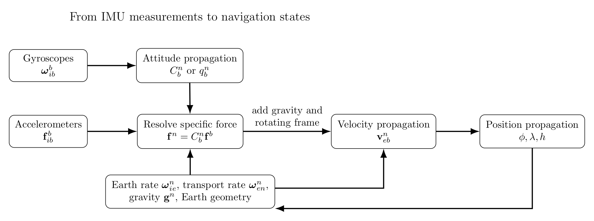
Figure. The strapdown navigation pipeline. Gyroscopes determine how the body frame
rotates; accelerometers measure specific force in that rotating body frame. Attitude is
therefore required before accelerometer measurements can be converted into
navigation-frame acceleration.
The treatment follows the physical and mathematical structure used in standard inertial-navigation
references, especially Titterton and Weston [1], Groves [2], Jekeli [3], and the modern
integration-algorithm treatment of Savage [4, 5].
1 Learning objectives
After completing this entry, the reader should be able to:
- explain what a strapdown inertial navigation system estimates and why integration is
required;
- distinguish a physical vector from the coordinates used to represent that vector;
- identify the inertial, Earth fixed, local navigation, and body frames used throughout
the series;
- interpret the notation Cbn, v
ebn, and ω
ibb;
- explain physically what an ideal gyroscope and an ideal accelerometer measure;
- explain why an accelerometer at rest on a table measures approximately one g even
though its translational acceleration is zero;
- state the complete attitude, velocity, and position mechanization equations that the
later lessons will derive;
- identify where Earth rotation, navigation frame transport, gravity, and Coriolis terms
enter the mechanization;
- explain why attitude error immediately contaminates translational navigation;
- describe the sequence of topics needed to progress from raw IMU data to a working
strapdown inertial navigator.
2 What inertial navigation is trying to estimate
For a vehicle moving near the Earth, the navigation problem is usually separated into three state
groups:
- attitude: orientation of the vehicle body frame relative to a chosen navigation frame;
- velocity: translational velocity of the vehicle relative to the Earth, resolved in the
navigation frame;
- position: location of the vehicle, often represented by latitude, longitude, and height.
In a local North-East-Down navigation frame, one common state description is
where Cbn describes attitude, v
ebn is Earth relative velocity resolved in the navigation frame, and
(ϕ,λ,h) are geodetic latitude, longitude, and ellipsoidal height.
The navigation computer does not measure these quantities directly. Its primary inertial inputs are
angular motion from the gyroscopes and specific force from the accelerometers.
3 Why the system is called strapdown
Early inertial navigation systems often mounted accelerometers on a mechanically stabilized
platform. Gyroscopes drove gimbals so that the sensor platform remained aligned with a useful
reference frame while the vehicle rotated around it. In that architecture the mechanical platform
performed much of the coordinate transformation physically.
A strapdown system removes the stabilized platform. The inertial measurement unit is rigidly
attached, or “strapped down,” to the vehicle. As a result, the sensors rotate whenever the vehicle
rotates. The coordinate transformation that once occurred mechanically must now be performed
mathematically in the navigation computer [1, 2].
This changes the problem fundamentally:
High rate digital computation and compact solid state sensors make the strapdown architecture
practical, but they also expose the navigator directly to finite rotation effects such as coning and
sculling. Those topics appear later in the series.
4 A vector is not the same thing as its coordinates
This distinction is essential throughout inertial navigation.
A physical vector, such as velocity v, exists independently of the coordinate frame used to describe
it. Its numerical components change when the basis changes. We therefore write a superscript to
indicate the frame in which the components are resolved:
for body frame components and
for navigation frame components.
The two component sets describe the same geometric vector and are related by a direction cosine
matrix:
Throughout this series, Cbn is a passive coordinate transformation: it maps components resolved in
frame b into components resolved in frame n.
Because the transformation represents an orthonormal rotation,
The detailed construction of direction cosine matrices and their relation to basis vectors is the
subject of INS01.
5 The four principal coordinate frames
A strapdown navigator near Earth commonly uses four frames.
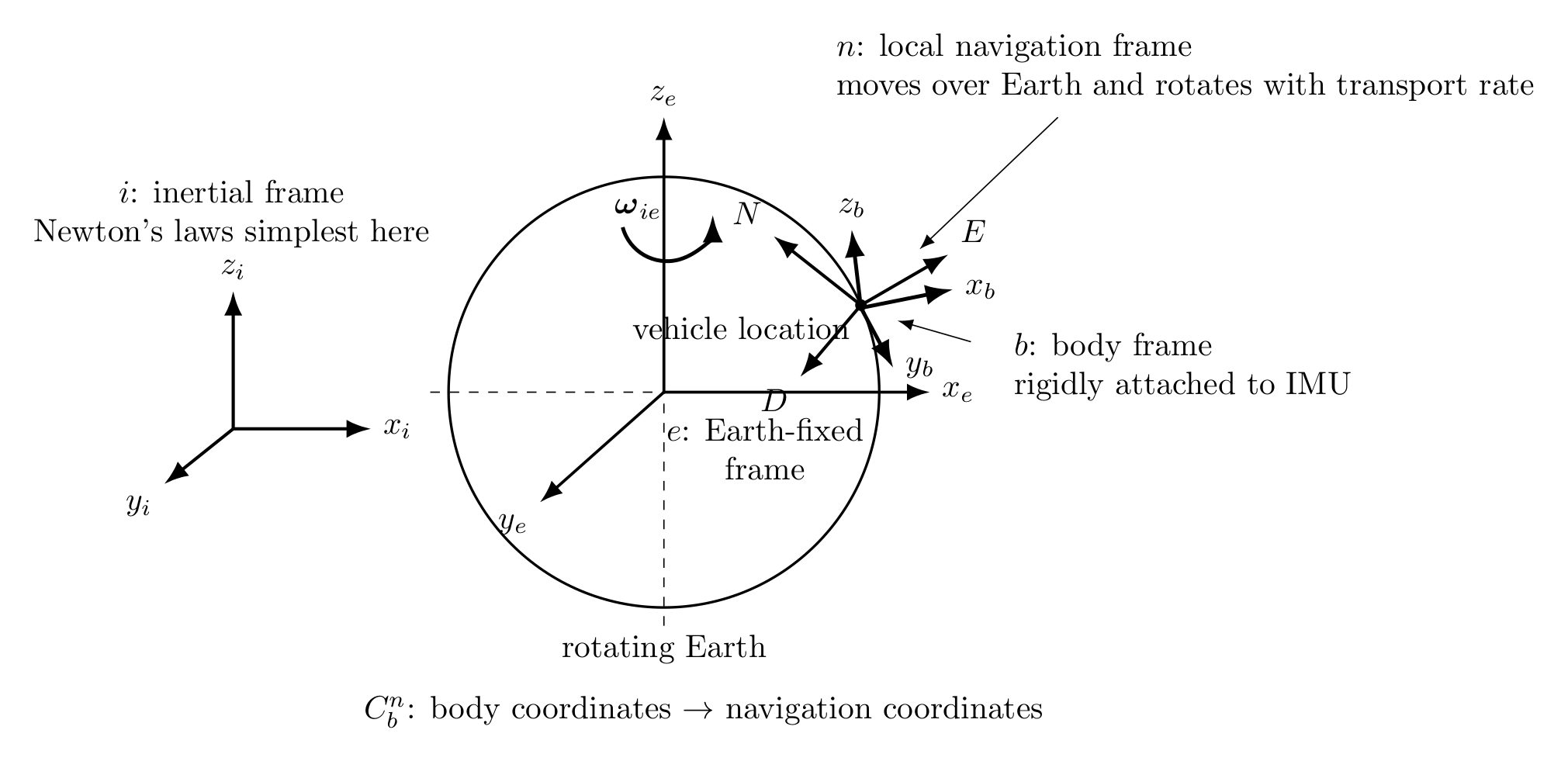
Figure. The principal frames used in the series. The body frame rotates with the vehicle,
the local navigation frame follows the vehicle over the rotating Earth, the Earth fixed
frame rotates with the Earth, and the inertial frame is the reference from which Newtonian
translational and rotational laws are most directly written.
5.1 Inertial frame i
The inertial frame is an ideal nonaccelerating, nonrotating frame suitable for Newton’s laws. In
practical terrestrial navigation an Earth centered inertial approximation is commonly used over the
relevant time scales.
The point of introducing i is conceptual as well as computational: gyroscopes fundamentally sense
body rotation relative to inertial space, and Newton’s second law has its cleanest form in an
inertial frame.
5.2 Earth frame e
The Earth centered, Earth fixed frame rotates with the Earth. Its origin is near the Earth’s center
of mass and its axes remain fixed relative to the terrestrial surface.
The Earth frame is therefore not inertial. Its angular velocity relative to the inertial frame is the
Earth rotation vector
The conventional Earth rotation magnitude used in navigation is approximately
which is about 15.04 degrees per hour.
5.3 Navigation frame n
The local navigation frame is attached to the vehicle’s current location. This series uses the
common North-East-Down convention:
Even if the Earth were not spinning, this frame would rotate as the vehicle moves over the curved
Earth. That motion generated angular rate is the transport rate.
Thus the navigation frame rotates relative to inertial space for two distinct reasons:
The first term is Earth rotation; the second is navigation frame transport due to motion over the
Earth.
5.4 Body frame b
The body frame is fixed to the vehicle and normally aligned with convenient vehicle axes. A
common aerospace convention is forward-right-down.
The IMU measurements are naturally resolved in this frame. Consequently, the navigator must
continuously estimate how b is oriented relative to n.
6 Angular rate notation
Angular velocity notation is a common source of confusion, so this series uses an explicit three
index convention:
It means:
angular velocity of frame b relative to frame a, resolved into coordinates of frame
c.
Examples are
for body rotation relative to inertial space, resolved in body coordinates, and
for Earth rotation relative to inertial space, resolved in the local navigation frame.
This explicit notation makes equations longer, but it prevents physically different angular rates
from being mistaken for one another.
7 What the gyroscopes measure
An ideal three axis gyroscope measures the angular velocity of the body frame relative to inertial
space, resolved in body coordinates:
A real gyro reports something closer to
The exact sensor error model is deferred to INS18.
The important physical point for now is that a gyro attached to an object sitting motionless on
Earth’s surface does not ideally read zero. The body is rotating through inertial space with the
Earth. In a sufficiently accurate gyro, Earth rotation is observable and can even be used for
heading alignment.
8 What the accelerometers measure
An accelerometer does not directly measure gravitational acceleration, and it does not directly
measure the coordinate acceleration d2r∕dt2.
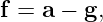
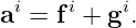
An ideal accelerometer measures specific force: the nongravitational force per unit mass acting on
the proof mass. In an inertial frame,
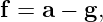
where a is inertial acceleration and g is gravitational acceleration.
The body mounted accelerometers provide body resolved specific force,
A real accelerometer measurement can be represented schematically as
8.1 The table top thought experiment
Suppose an accelerometer rests on a table. Its translational acceleration relative to the table is
approximately zero, yet the accelerometer reads approximately one g upward along the local
vertical axis.
Why?
Gravity pulls the accelerometer proof mass downward, while the housing and support structure
exert an upward contact force that prevents free fall. The accelerometer senses the nongravitational
support force per unit mass.
By contrast, in ideal ballistic free fall,
so
The proof mass becomes locally weightless and the accelerometer ideally reads zero.
This distinction between gravity and specific force is one of the central physical ideas in inertial
navigation and is developed carefully in INS03.
9 Why attitude must be solved before translational acceleration
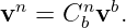
Accelerometers report fb, but the velocity state is normally maintained in another frame such as
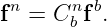
NED or ECEF. Therefore the specific force vector must be transformed:
This simple equation explains why attitude errors are so dangerous. If Cbn is wrong, the navigator
resolves the measured force into the wrong directions.
A small tilt error δ𝜃 causes a component of the approximately vertical gravity supporting specific
force to leak into a horizontal channel. For small angles,
Thus even a tiny attitude error can produce a persistent false horizontal acceleration.
INS19 will turn this observation into a complete linear error model and derive Schuler
dynamics.

Figure. A representative inertial error chain. Gyro error first becomes attitude error;
attitude error then misprojects specific force and gravity, creating false acceleration that
integrates into velocity and position error.
10 The simplest navigation equation: inertial frame first
Before Earth rotation and local level geometry are introduced, the translational mechanics are
remarkably simple.
Newton’s second law per unit mass is
Since the accelerometers measure specific force in body coordinates,
Therefore
This is the conceptual core of strapdown translational navigation:
The complexity of terrestrial navigation arises because practical coordinates such as ECEF and
NED are themselves rotating and because gravity is not perfectly uniform.
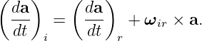
11 The rotating frame problem
If a vector is differentiated in a rotating frame, its time derivative differs from the derivative seen
in an inertial frame. The fundamental transport theorem is
Applying this relation repeatedly to position and velocity produces the familiar noninertial
acceleration terms:
and, when the rotation rate itself changes,
These become the Coriolis, centrifugal, and Euler acceleration terms. INS02 derives them from
rotating basis vectors rather than introducing them by name.
12 The three equations the series is building toward
The rest of the course derives and implements three coupled differential equations: attitude,
velocity, and position.
12.1 Attitude equation
With the passive transformation convention used here,
The skew-symmetric matrix [a]× is defined so that
The first term propagates body rotation measured by the gyroscopes. The second accounts for
rotation of the navigation frame itself.
Since
the attitude solution must ultimately compensate both Earth rotation and transport
rate.
INS07 derives the DCM equation, while INS08 derives the equivalent quaternion propagation
equation.
12.2 Velocity equation
For an Earth relative velocity maintained in NED coordinates, the standard local level
mechanization has the form
Every term has a physical origin:
- Cbnf
ibb: measured specific force rotated from body coordinates into navigation
coordinates;
- gn: gravity restored because accelerometers do not measure gravity directly;
- 2ωien × v
ebn: Coriolis acceleration associated with Earth rotation;
- ωenn × v
ebn: correction associated with rotation of the local navigation frame as it
moves over Earth.
Depending on the exact gravity definition, centrifugal effects are conventionally absorbed into the
gravity model. INS05 and INS11 make that bookkeeping explicit.
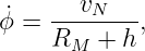
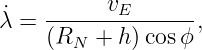
12.3 Position equation
For geodetic latitude ϕ, longitude λ, and ellipsoidal height h,
and, with NED coordinates,
Here RM and RN are the meridian and prime vertical radii of curvature of the reference
ellipsoid.
These relations are not arbitrary conversion formulas. They follow from Differential Geometry of
motion over the ellipsoid and are derived in INS14.
13 The mechanization is a coupled feedback process
The attitude, velocity, and position equations cannot be solved independently.
Position determines latitude and height, which influence gravity and the resolved Earth rotation
rate. Velocity and position determine transport rate. Earth rate and transport rate enter
attitude propagation. Attitude determines how measured specific force is projected
into the navigation frame. That projected force changes velocity, and velocity changes
position.
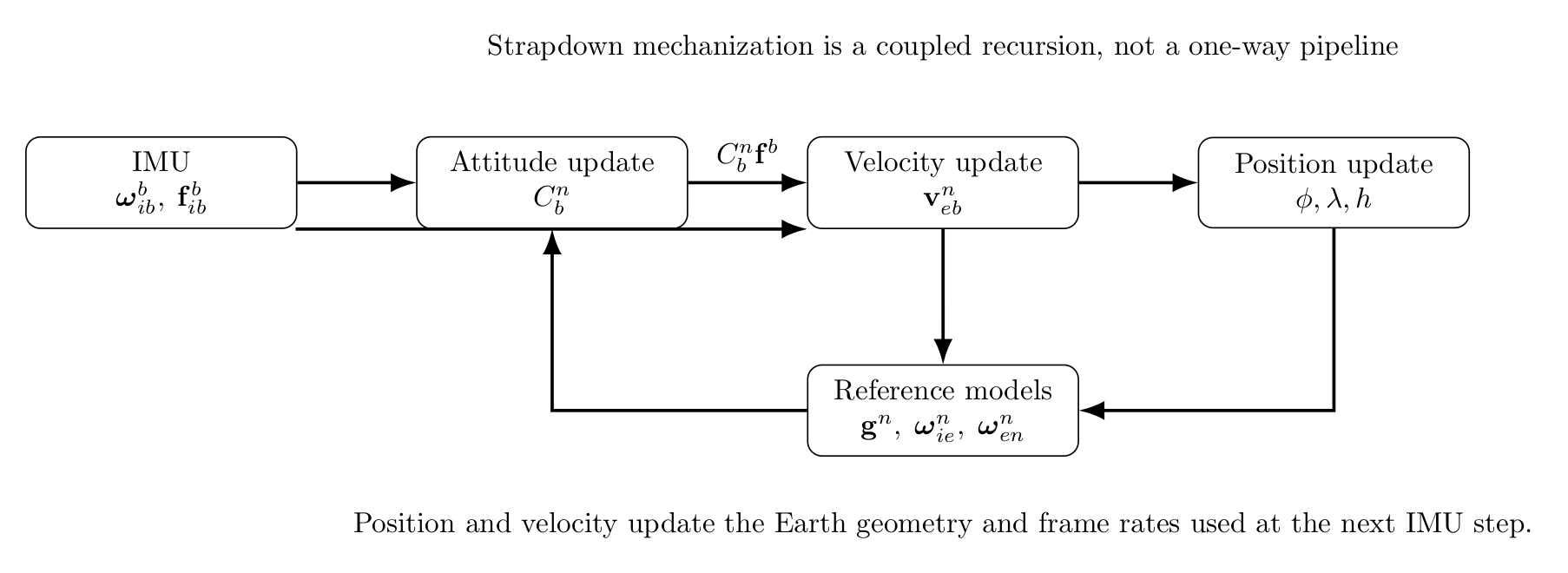
Figure. The strapdown mechanization loop. The apparent left-to-right processing chain is
actually coupled: position and velocity feed the reference frame rates and gravity model
used in the next attitude and velocity update.
This coupling is why consistent frame notation and timing are essential in implementation.
14 Continuous equations versus actual IMU data
The differential equations above are mathematically continuous. A real digital IMU normally
delivers sampled data, often as increments over a finite time interval:
from the gyroscopes and
from the accelerometers.
Therefore a working navigator must approximate the continuous dynamics over each finite sample
interval. Straightforward first order integration is not always sufficient because finite
rotations do not commute and because translational increments occur while the body is
rotating.
This leads to the advanced strapdown corrections:
- coning corrections for accumulated rotation;
- sculling corrections for velocity increments acquired under rotation;
- high resolution position corrections sometimes called scrolling in the strapdown
literature.
Savage’s two part integration algorithm treatment is a standard source for these subjects [4, 5].
They are deferred to INS16 and INS17 so the continuous physics is fully understood
first.
15 What a pure INS can and cannot know
A strapdown INS is a dead reckoning system. Once initialized, it can propagate motion without
receiving an external signal. This gives it excellent short term continuity and makes it resistant to
radio frequency outages.
However, integration also accumulates sensor error. Biases in gyroscopes and accelerometers do not
average away automatically. Instead they drive growing errors in attitude, velocity, and
position.
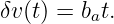
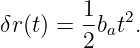
A simple accelerometer bias example illustrates this. If a constant horizontal acceleration error ba is
integrated once,
Integrating again gives
Gyro bias can be even more damaging because it first creates attitude error and then misprojects
gravity into the horizontal channels.
Consequently, practical navigation systems commonly aid the INS with GNSS, barometers,
magnetometers, odometers, cameras, radar, lidar, or other external measurements. Those aiding
systems do not replace the strapdown mechanization; they estimate and correct its
errors.
This course deliberately postpones Kalman filtering until the deterministic mechanization and
error physics are understood.
16 Three thought experiments to carry through the series
16.1 Stationary IMU on the Earth
A motionless IMU on a laboratory table is not dynamically trivial.
Its accelerometers measure the support specific force associated with gravity, while sufficiently
sensitive gyroscopes measure Earth rotation. A correct mechanization should nevertheless maintain
nearly zero Earth relative velocity and fixed position after alignment.
This is one of the most useful numerical acceptance tests for a strapdown navigator.
16.2 IMU in free fall
In ideal free fall,
The accelerometers therefore read zero even though the vehicle accelerates gravitationally. The
navigation computer must recover gravitational acceleration from its gravity model.
This thought experiment is the clearest test of the difference between acceleration and specific
force.
16.3 Vehicle undergoing pure rotation
Suppose the vehicle rotates in place without translating. The gyroscopes measure angular motion,
the attitude changes, but the true velocity and position remain fixed.
A correct mechanization must continuously rotate the measured support specific force vector while
still producing zero translational motion after gravity and rotating frame terms are handled
consistently.
This example exposes attitude sign, frame order, and gravity projection mistakes very
quickly.
17 Series roadmap
The Strapdown Inertial Navigation series is organized so that each term in the final mechanization
equations is derived from simpler physics before it is implemented.
|
|
|
ID | Topic | Main purpose |
|
|
|
INS00 | Roadmap, frames, and
notation | Establish the complete problem and
the target equations. |
INS01 | Vectors, frames, and DCMs | Separate physical vectors
from coordinates and construct passive
transformations. |
INS02 | Derivatives in rotating frames | Derive transport theorem, Coriolis,
centrifugal, and Euler terms. |
INS03 | Accelerometer physics | Derive specific force and explain
support force versus free fall. |
INS04 | Gyroscope physics | Interpret
inertial angular rate measurements and
practical gyro outputs. |
INS05 | Gravitation and gravity | Build from Newtonian gravitation to
rotating Earth Normal gravity. |
INS06 | Earth rotation and local
frames | Resolve Earth rate and establish ECI,
ECEF, and NED relationships. |
INS07 | DCM attitude propagation | Derive the strapdown attitude
differential equation. |
INS08 | Quaternion propagation | Derive quaternion kinematics and
incremental rotation updates. |
INS09 | Initial alignment | Recover level and heading information
from gravity and Earth rate. |
INS10 | Inertial frame translation | Derive the clean Newtonian specific
force navigation equation. |
INS11 | Rotating Earth dynamics | Derive Earth frame Coriolis and
centrifugal effects. |
INS12 | ECEF mechanization | Build a complete Cartesian Earth fixed
strapdown navigator. |
INS13 | Navigation frame transport
rate | Derive local frame rotation caused by
motion over curved Earth. |
INS14 | Ellipsoidal position kinematics | Derive latitude, longitude, and height
rates from local velocity. |
INS15 | Complete NED mechanization | Assemble attitude, velocity, position,
gravity, Earth rate, and transport rate. |
INS16 | Discrete IMU mechanization | Convert continuous equations to finite
rate sampled updates. |
INS17 | Coning and sculling | Treat noncommuting rotations and
rotating frame velocity increments. |
INS18 | IMU calibration and errors | Introduce bias, scale
factor, misalignment, temperature, and
stochastic errors. |
INS19 | INS error dynamics | Derive error growth and Schuler
dynamics before filtering. |
INS20 | Computational laboratory | Implement and
validate the full mechanization against
synthetic truth. |
|
|
|
18 A notation reference for the rest of the series
|
|
Symbol | Meaning |
|
|
i | inertial frame |
e | Earth centered, Earth fixed frame |
n | local navigation frame; NED in this series |
b | body frame fixed to the vehicle |
Cbn | passive DCM mapping body resolved components into
navigation frame components |
vebn | velocity of body b relative to Earth frame e, resolved in frame
n |
ωabc | angular velocity of frame b relative to frame a, resolved in
frame c |
fibb | specific force of body relative to inertial dynamics, resolved
in body coordinates |
gn | gravity vector used by the mechanization, resolved in frame
n |
[a]× | skew matrix satisfying [a]×b = a × b |
ϕ,λ,h | geodetic latitude, longitude, and ellipsoidal height |
RM,RN | meridian and prime vertical radii of curvature |
|
|
19 Implementation discipline
Several habits will be maintained throughout the series because they prevent common strapdown
navigation errors.
- Every vector quantity carries an explicit resolving frame until the context is completely
unambiguous.
- Every angular velocity identifies both frames and the resolving frame.
- The passive DCM convention is not changed between articles.
- NED uses positive Down, so ḣ = −vD.
- Gravity model definitions state explicitly whether centrifugal effects are included.
- Continuous time derivations are separated from sampled data algorithms.
- Analytic or synthetic truth cases are used before complicated flight data.
- Every mechanization implementation is tested first with stationary, pure rotation, and
simple constant acceleration cases.
These conventions are not stylistic decoration. Most implementation failures in inertial navigation
are ultimately frame, sign, timing, or model consistency errors.
20 Summary
A strapdown INS reconstructs navigation states from body fixed measurements. Its ideal
measurements are
from the gyroscopes and
from the accelerometers.
The central physical relationship for translation is
so specific force must be transformed into the navigation frame and combined with an appropriate
gravity model before velocity can be propagated.
The local level attitude equation is
with
The corresponding NED velocity equation is
Position is propagated through ellipsoidal geometry:
The remaining articles derive each of these relationships from first principles, then convert them
into a discrete strapdown algorithm that can be validated numerically.
References
[1] David H. Titterton and John L. Weston, Strapdown Inertial Navigation Technology,
2nd ed., Institution of Electrical Engineers, 2004.
[2] Paul D. Groves, Principles of GNSS, Inertial, and Multisensor Integrated Navigation
Systems, 2nd ed., Artech House, 2013.
[3] Christopher Jekeli, Inertial Navigation Systems with Geodetic Applications, Walter
de Gruyter, 2001.
[4] Paul G. Savage, “Strapdown Inertial Navigation Integration Algorithm Design Part
1: Attitude Algorithms,” Journal of Guidance, Control, and Dynamics, Vol. 21, No. 1,
pp. 19–28, 1998.
[5] Paul G. Savage, “Strapdown Inertial Navigation Integration Algorithm Design Part
2: Velocity and Position Algorithms,” Journal of Guidance, Control, and Dynamics, Vol.
21, No. 2, pp. 208–221, 1998.

























![dCn
---b-= Cnb [ωbib]× − [ωnin]×Cnb .
dt](https://images.physicslibrary.org/cache/objects/1343/make4ht/StrapdownInertialNavigationRoadmapFramesAndTheMechanizationProblem31x.png)
![[a]×b = a × b.](https://images.physicslibrary.org/cache/objects/1343/make4ht/StrapdownInertialNavigationRoadmapFramesAndTheMechanizationProblem32x.png)






![n
dC-b-= Cn [ωb ]× − [ωn ]×Cn ,
dt b ib in b](https://images.physicslibrary.org/cache/objects/1343/make4ht/StrapdownInertialNavigationRoadmapFramesAndTheMechanizationProblem46x.png)


