Constant Acceleration Motion
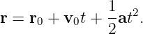
Constant acceleration motion is motion for which the acceleration remains unchanged during the
time interval being studied. In one dimension,
This simple condition produces one of the most important families of equations in introductory
mechanics. Because acceleration is the time derivative of velocity, and velocity is the time
derivative of position, the constant acceleration equations follow directly by integration.
The results are not independent formulas to memorize. They are different algebraic forms of the
same underlying kinematics.
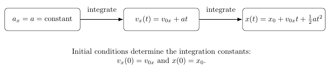
Figure 1. Constant acceleration integrates once to a linear velocity law and a second time to a
quadratic position law. The initial position and velocity determine the integration constants.
1 Assumptions and scope
For one-dimensional motion, the constant acceleration model assumes
where a does not vary with time over the interval of interest.
The model applies exactly to idealized cases such as a particle moving under a constant net force
with constant mass. It also provides an excellent approximation for many short-duration problems
in which the acceleration changes negligibly.
It does not apply without modification when acceleration depends appreciably on time, position, or
velocity. Examples include strong aerodynamic drag, a spring force over a large interval, or gravity
over distances large enough that g changes significantly.
2 Derivation of the velocity equation
Acceleration is defined by
For constant a,
Integrate from the initial state at t = 0, where the velocity is v0x, to a later time t:
Therefore
or
The velocity therefore changes linearly with time. On a velocity-time graph, the slope is the
constant acceleration.
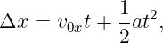
3 Derivation of the position equation
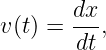
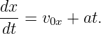
Velocity is
Insert the constant acceleration velocity law:
Thus
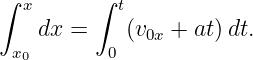
Integrating from x0 at t = 0 to x at time t gives
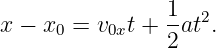
Hence
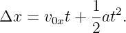
Using the displacement Δx = x − x0,
Because the position contains a term proportional to t2, the position-time graph is parabolic when
acceleration is nonzero.
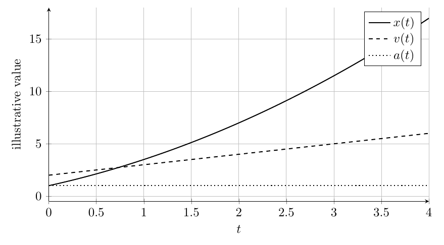
Figure 2. For constant positive acceleration, acceleration is horizontal on an acceleration-time
graph, velocity changes linearly, and position is quadratic in time. The plotted values are
illustrative rather than dimensionally identical.
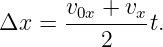
4 Average velocity for constant acceleration
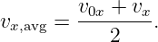
When acceleration is constant, the velocity changes linearly with time. The average
value of a linear function over an interval is the arithmetic mean of its endpoint values.
Therefore
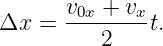
Since displacement equals average velocity times elapsed time,
This result is specific to constant acceleration. It is not generally true when acceleration varies with
time.
5 Eliminating time
Some problems give positions and velocities but not the elapsed time. Time can be eliminated
algebraically.
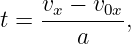
From
we have
provided a≠0.
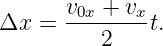
Insert this into
Then
Using
we obtain
This form is especially useful when time does not appear among the known or requested
quantities.
6 The four standard one-dimensional relations
For constant acceleration in one dimension, the most useful equations are
and
These equations contain the same physical information. Which form is most convenient depends on
which variables are known.
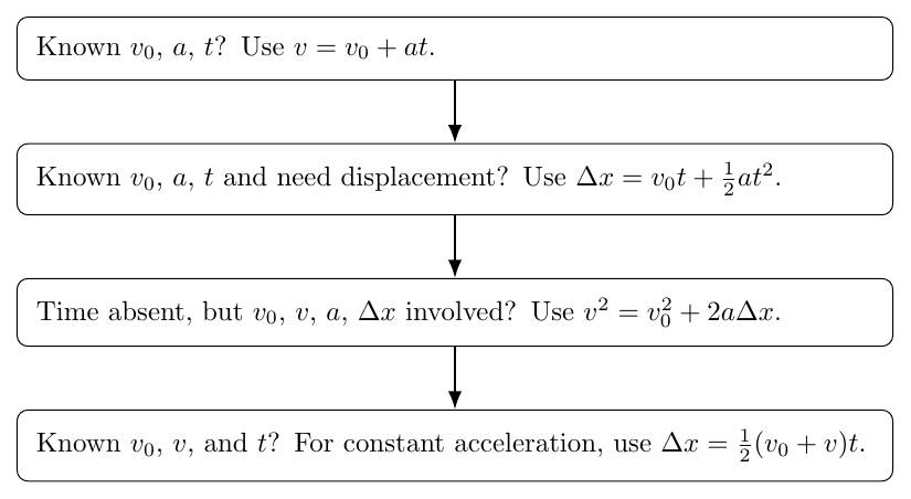
Figure 3. A practical equation-selection map. List the known quantities and choose a relation that
contains the unknown but omits a variable that is neither known nor needed.
7 Sign conventions
The equations are vector-consistent only when signs are assigned according to a chosen positive
direction.
For one-dimensional motion, choose the positive axis first. Then:
- velocity is positive when motion is in the positive direction;
- velocity is negative when motion is in the negative direction;
- acceleration is positive when the acceleration vector points in the positive direction;
- acceleration is negative when it points in the negative direction;
- displacement is positive or negative according to the final position relative to the initial
position.
A negative acceleration does not automatically mean that an object is slowing down. An object
speeds up when velocity and acceleration have the same sign and slows down when they have
opposite signs.
8 Vertical motion near Earth’s surface
When aerodynamic drag is neglected and the vertical range is small compared with Earth’s radius,
gravitational acceleration near the surface is approximately constant.
Choose upward as positive. Then
where
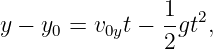
The constant acceleration equations become
and
At the highest point of an upward throw,
but the acceleration is still

Figure 4. With upward chosen as positive, gravitational acceleration is negative throughout the
flight. At maximum height the vertical velocity is momentarily zero, but the acceleration remains
downward.
A downward-positive coordinate system is equally valid. In that convention ay = +g. The physics
is unchanged as long as one convention is used consistently.
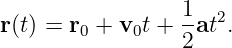
9 Vector form
For motion in several dimensions with a constant acceleration vector a, the one-dimensional
relations generalize componentwise:
and
Thus each Cartesian component obeys its own constant acceleration equation. Projectile motion is
an important application: with negligible air resistance, the horizontal acceleration is
approximately zero and the vertical acceleration is approximately −g.
10 Dimensional checks
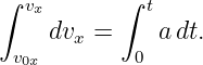
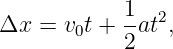
Every term in a kinematic equation must have the same dimensions.
For
we have
and
Similarly, in
both v2 and aΔx have dimension L2∕T2.
Dimensional consistency cannot prove that an equation is correct, but it can quickly expose many
algebraic errors.
11 Worked example 1: braking to rest
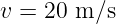
A CAR travels at
and brakes with constant acceleration
Find the stopping time and stopping distance.
Choose the initial direction of motion as positive. At rest,
Using
we get
so
The displacement is
which gives
The negative acceleration describes braking because the velocity is initially positive.
12 Worked example 2: ball thrown vertically upward
A ball is launched upward from y0 = 0 with
Neglect air resistance. Find the time to maximum height, the maximum rise, and the time to
return to the launch height.
Choose upward as positive, so
At the top,
Therefore
so
Use the no-time equation for the rise:
Hence
Because the ball returns to its launch height under constant downward acceleration with no drag,
the ascent and descent times are equal. Thus
At that instant the velocity is approximately −18.0 m/s. The speed magnitude equals the launch
speed, but the direction is downward.
13 Worked example 3: two-dimensional constant acceleration
A particle has
and constant acceleration
Find the velocity and position at t = 3.0 s.
The velocity is
so
or
The position is
Thus
The displacement is therefore
with magnitude
14 Worked example 4: find acceleration without finding time first
A vehicle speeds up uniformly from
to
over a displacement of
Find the acceleration and elapsed time.
Because time is not initially known, use
Then
so
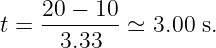
Now use
to obtain
This example illustrates why equation selection should follow the available variables rather than a
fixed memorized order.
15 Common mistakes
- Using the constant acceleration equations when acceleration actually varies
significantly.
- Substituting the magnitude g without first deciding whether it is positive or negative
in the chosen coordinate system.
- Assuming negative acceleration always means slowing down.
- Assuming that v = 0 implies a = 0 at the top of vertical motion.
- Mixing position x with displacement Δx = x − x0.
- Using Δx = (v0 + v)t∕2 when the acceleration is not constant.
- Forgetting that the equation v2 = v
02 + 2aΔx loses the sign of v when one later takes
a square root.
16 Practice problems
M01-05-P01
A particle begins with v0 = 3.0 m∕s and has constant acceleration a = 2.0 m∕s2. Find its velocity
after 5.0 s.
M01-05-P02
A car starts from rest and accelerates at 3.0 m∕s2 for 6.0 s. Find its displacement.
M01-05-P03
A cyclist moving at 12 m∕s slows uniformly at −2.0 m∕s2. Find the time required to reach
4.0 m∕s.
M01-05-P04
A train speeds up uniformly from 8 m∕s to 20 m∕s in 6.0 s. Find its acceleration and
displacement.
M01-05-P05
A car traveling at 30 m∕s brakes uniformly at −5.0 m∕s2. Find the stopping distance.
M01-05-P06
A stone is dropped from rest. Neglect air resistance and take downward as positive. Find its speed
and downward displacement after 2.0 s using g = 9.81 m∕s2.
M01-05-P07
A ball is thrown straight upward at 14 m∕s. Take upward as positive. Find the time to the highest
point and the maximum rise.
M01-05-P08
A particle has x0 = −4 m, v0 = 5 m∕s, and a = −1.5 m∕s2. Find x and v at t = 4.0
s.
M01-05-P09
A vehicle covers 72 m while accelerating uniformly from 6 m∕s to 18 m∕s. Find the
acceleration.
M01-05-P10
A particle moving at −10 m∕s has acceleration −2.0 m∕s2 for 3.0 s. Is it speeding up or slowing
down? Find its final velocity.
M01-05-P11
A particle has v0 = 2ex + 3ey m∕s and a = 4ex − 2ey m∕s2. Find v after 2.0 s.
M01-05-P12
A ball is released from rest from a height of 19.6 m above the ground. Neglect air resistance and
use g = 9.8 m∕s2. Find the time to reach the ground and the speed immediately before
impact.
17 Compact answer check
- 13 m∕s.
- 54 m.
- 4.0 s.
- 2.0 m∕s2 and 84 m.
- 90 m.
- 19.6 m∕s and 19.6 m downward.
- 1.43 s and approximately 10.0 m.
- x = 4 m and v = −1 m∕s.
- 2.0 m∕s2.
- Speeding up; v = −16 m∕s.
- v = 10ex − 1ey m∕s.
- 2.0 s and 19.6 m∕s.
18 Connection to the next article
Constant acceleration is special because integration gives simple polynomial functions of time.
M01-06 removes that restriction and studies variable acceleration, for which one must work directly
with
and
or with position-dependent and velocity-dependent forms of acceleration.
References
[1] PhysicsLibrary, M01-01: Position and Displacement in Mechanics.
[2] PhysicsLibrary, M01-02: Velocity in Mechanics.
[3] PhysicsLibrary, M01-03: Acceleration in Mechanics.
[4] PhysicsLibrary, M01-04: Motion Graphs in Kinematics.
[5] PhysicsLibrary, Constant Acceleration Problems, existing example material.
[6] OpenStax / cnxuniphysics, University Physics Volume 1, archived 2016 BCcampus
clone, CC BY 4.0.
[7] University of California, Davis, Physics 9A: Classical Mechanics, Physics LibreTexts,
CC BY-SA 4.0.
[8] J. R. Taylor, Classical Mechanics, University Science Books, 2005. Used as a scope
and notation reference.






















![[v0t] = (L∕T )T = L,](https://images.physicslibrary.org/cache/objects/1316/make4ht/ConstantAccelerationMotion35x.png)
![[at2] = (L∕T 2)T2 = L.](https://images.physicslibrary.org/cache/objects/1316/make4ht/ConstantAccelerationMotion36x.png)