Variable Acceleration Motion
Variable acceleration motion occurs when acceleration changes during the interval being studied.
The acceleration may depend on time, position, velocity, or several variables at once. In such
problems the familiar constant acceleration equations are generally not valid. Instead, one returns
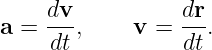
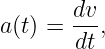
to the differential definitions
and
and integrates or solves the resulting differential equations using the supplied acceleration law and
initial conditions.
The essential idea is simple: acceleration tells how velocity changes, and velocity tells how position
changes. When acceleration is variable, those changes must be accumulated with calculus rather
than represented by one constant slope.
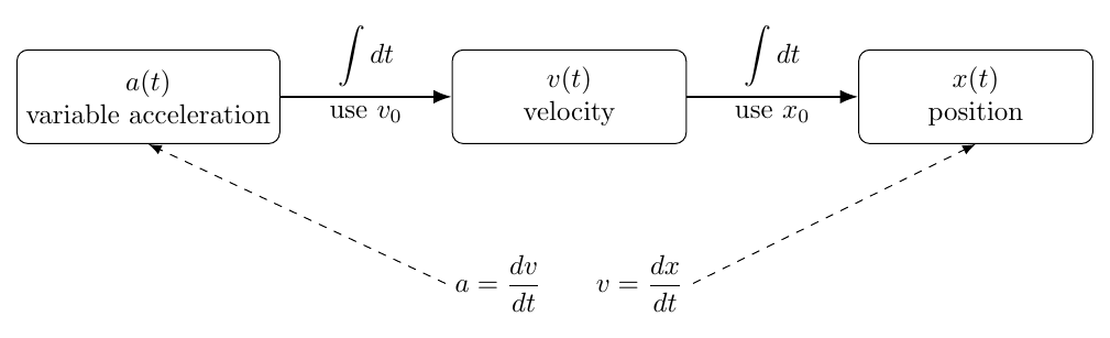
Figure 1. Variable acceleration is accumulated by integration. Integrating the acceleration law
gives velocity, and integrating the velocity gives position. Initial conditions determine the
constants of integration.
1 Why the constant acceleration equations stop working
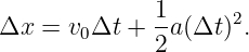
For constant acceleration one may write
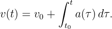
If acceleration varies with time, however, the quantity at no longer represents the accumulated
change in velocity. The correct relation is
Likewise, the displacement is not generally
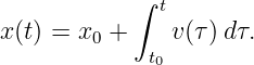
Instead,
The constant acceleration equations are therefore special cases of the more general integral
relations.
2 Time dependent acceleration
Suppose one-dimensional acceleration is known explicitly as a function of time:
Since
we have
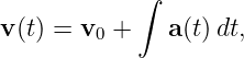
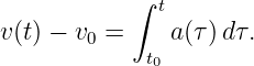
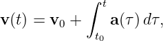
Integrating from an initial time t0 with velocity v0 to a later time t gives
The dummy variable τ is used inside the integral so that the upper limit t remains distinct from
the integration variable.
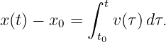
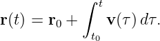
Once v(t) is known,
Thus a known a(t) is integrated twice to obtain position.
3 A double integral form
Substituting the velocity integral into the position integral gives
For most introductory problems it is clearer to integrate in two separate steps, but the double
integral form makes the structure explicit: variable acceleration is accumulated once into velocity
and again into position.
4 Geometric interpretation on motion graphs
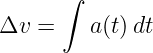
On an acceleration time graph,
is the signed area under the acceleration curve.
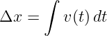
On a velocity time graph,
is the signed area under the velocity curve.
The graphical and calculus viewpoints are the same statement in different forms.
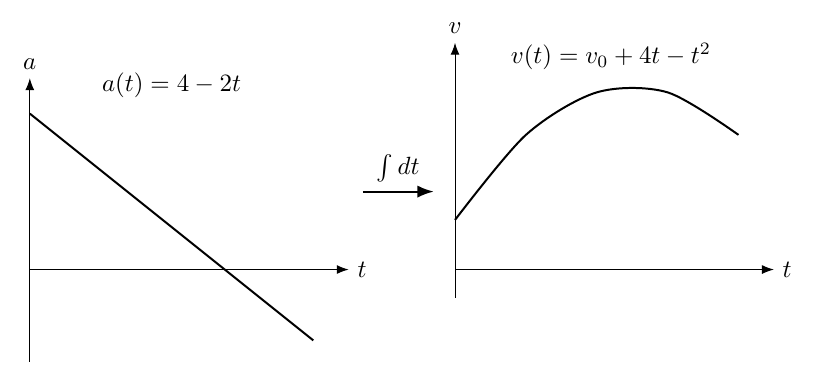
Figure 2. Example of time dependent acceleration. The changing acceleration produces a curved
velocity graph; integrating again produces the position history.
5 Acceleration given as a function of position
Sometimes acceleration is specified as a function of position rather than time:
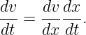
The definition
contains a time derivative, but the chain rule can eliminate time:
Since
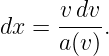
we obtain the fundamental one-dimensional identity
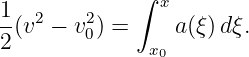
Therefore
Integrating from (x0,v0) to (x,v) gives
This relation is especially useful when time is absent from the problem.
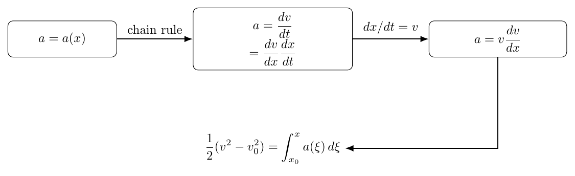
Figure 3. If acceleration is supplied as a function of position, the chain rule converts the time
derivative into the useful form a = v dv∕dx.
6 Connection with the constant acceleration no time equation
If a(x) = a0 is constant, then
Multiplying by two gives
Thus the familiar no time constant acceleration equation is a special case of the variable position
relation.
7 Acceleration given as a function of velocity
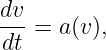
A prescribed kinematic model may also have
Because
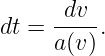
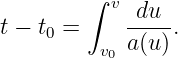
one may separate variables when a(v)≠0:
Hence
Using a = v dv∕dx also gives
These forms become important later when forces such as aerodynamic drag produce acceleration
that depends on speed. In the present article the emphasis remains kinematic: the acceleration law
is assumed to be given.
8 Vector form for time dependent acceleration
If the acceleration vector is known as a function of time,
then
and
In a fixed Cartesian basis these vector integrals are evaluated component by component.
9 Initial conditions and constants of integration
Indefinite integration introduces constants. For example, if
then
and
The initial conditions determine C1 and C2. Using definite integrals usually makes this
bookkeeping more transparent because the initial values enter directly.
10 Turning points and sign information
A turning point in one-dimensional motion occurs when
and the velocity changes sign. Variable acceleration can produce several such points.
The equation v = 0 identifies candidate turning times or positions, but one should check the
velocity on either side. A zero of velocity need not be a reversal if the velocity only touches zero
and retains the same sign.
Similarly, the sign of acceleration alone does not determine whether the particle speeds up or slows
down. Speed increases when velocity and acceleration have the same sign and decreases when their
signs are opposite.
11 Piecewise acceleration
Realistic simplified models often specify different acceleration laws on different intervals. The
solution must then be propagated continuously from one interval to the next.
If the first interval ends at t = t1, compute
and use those values as the initial conditions for the next interval. Position and velocity are
normally continuous unless the idealized model explicitly introduces an instantaneous
impulse.
12 Numerical integration preview
Not every acceleration law has a convenient elementary antiderivative. Even when the acceleration
is known exactly, one may need numerical integration.
Over a small time step Δt, a basic approximation is
This is the forward Euler method. It is easy to understand but may require very small time steps
for good accuracy. Later computational mechanics articles can introduce more accurate schemes
such as midpoint and Runge–Kutta methods.
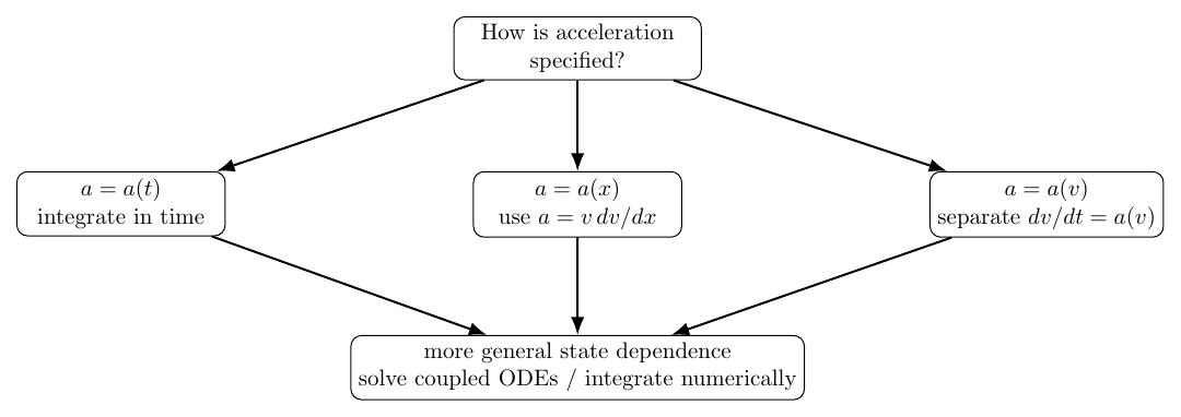
Figure 4. Choosing the constant acceleration method begins by asking what the acceleration is
given as a function of: time, position, velocity, or a more general state.
13 Worked example 1: acceleration varying linearly with time
A particle moves along the x axis with
At t = 0,
Find v(t) and x(t), then evaluate them at t = 3 s.
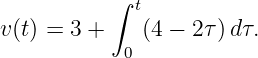
Integrate the acceleration:
Thus
Integrate velocity:
so
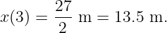
At t = 3 s,
and
The acceleration has changed from +4 m∕s2 initially to −2 m∕s2 at t = 3 s, yet the velocity is
still positive because velocity depends on the accumulated acceleration history.
14 Worked example 2: acceleration proportional to time
A particle has
with
Find the velocity and position at t = 4 s.
Integrating,
Therefore
Now integrate velocity:
Thus
15 Worked example 3: position dependent acceleration
A particle moves along the x axis with
where the numerical coefficient has units of s−2. At
it is momentarily at rest. Find its velocity when it reaches
Use
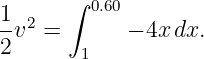
Then
Integrate from (x0,v0) = (1, 0) to (0.60,v):
Therefore
so
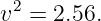
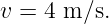
The speed is 1.60 m∕s. Because the particle began at positive x with acceleration toward
decreasing x, its velocity on the first inward pass is
The sign is supplied by the direction of motion; the integrated equation determines
v2.
16 Worked example 4: vector variable acceleration
A particle has
with
and
Find v and r at t = 2 s.
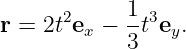
Integrating componentwise,
Thus
Integrating again,
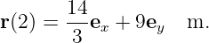
At t = 2 s,
17 Practice problems
M01-06-P01
A particle has a(t) = 6t m/s2, v(0) = 2 m/s, and x(0) = 1 m. Find v(t) and x(t).
M01-06-P02
A particle has a(t) = 3 − 4t m/s2 and v(0) = −1 m/s. Find the velocity at t = 2 s.
M01-06-P03
For a(t) = 2t2 m/s2 with v(0) = 0 and x(0) = 0, find the position at t = 3 s.
M01-06-P04
A one-dimensional particle has velocity v(t) = 5 + 2t − t2 m/s. Find its acceleration and identify
the time at which the acceleration changes sign.
M01-06-P05
A particle begins with v0 = 4 m/s. Its acceleration is +2 m/s2 from t = 0 to 3 s and then −1 m/s2
from t = 3 to 7 s. Find its final velocity.
M01-06-P06
For a(x) = 3x with x in meters and the coefficient in s−2, a particle has v
0 = 2 m/s at x0 = 0. Find
its speed at x = 2 m.
M01-06-P07
A particle satisfies a(x) = −9x and is released from rest at x0 = 0.50 m. Find its speed when it
first reaches x = 0.
M01-06-P08
Show that if a(x) = a0 is constant, integrating a = v dv∕dx gives v2 = v
02 + 2a
0(x − x0).
M01-06-P09
A particle has a(t) = 4ex − 2tey m/s2 and starts from rest at the origin. Find v(t) and
r(t).
M01-06-P10
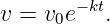
A velocity dependent acceleration is a(v) = −kv, where k is a positive constant with units s−1.
Starting from dv∕dt = −kv, separate variables and show that v(t) = v0e−kt.
18 Compact answer check
M01-06-P01:
M01-06-P02:
M01-06-P03:
M01-06-P04:
so a = 0 at t = 1 s.
M01-06-P05:
M01-06-P06:
M01-06-P07:
M01-06-P08: result as stated.
M01-06-P09:
M01-06-P10:
19 Common mistakes
- Using the four constant acceleration equations when a varies appreciably.
- Forgetting the initial condition constants after indefinite integration.
- Treating a(x) as though it could be integrated directly with respect to time without
first relating x and t.
- Using a = v dv∕dx without recognizing that it is a one-dimensional chain rule result.
- Taking the positive square root of v2 automatically; the sign of velocity must agree
with the actual direction of motion.
- Confusing zero acceleration at one instant with constant velocity over the entire motion.
20 Summary
Variable acceleration kinematics returns to the definitions
For time dependent acceleration,
followed by integration of velocity to obtain position. For one-dimensional position dependent
acceleration, the chain rule gives
which removes time and relates speed directly to position. These ideas form the natural extension
of constant acceleration kinematics and prepare for variable force dynamics, oscillations, drag, and
numerical integration.
References
[1] J. R. Taylor, Classical Mechanics, University Science Books, 2005. Used as a scope
and notation reference; prose and figures in this entry are original.
[2] J. W. Schnick, Calculus-Based Physics I, Open Textbook Library / BCcampus
collection, CC BY-SA 3.0.
[3] University of California, Davis, Physics 9A: Classical Mechanics, LibreTexts, CC
BY-SA 4.0.
[4] OpenStax, University Physics Volume 1, archived 2016 BCcampus revision, CC BY
4.0.






![[ ]
∫ t ∫ τ
x(t) = x0 + v0(t − t0) + a(s)ds dτ.
t0 t0](https://images.physicslibrary.org/cache/objects/1318/make4ht/VariableAccelerationMotion11x.png)


































![1
-v2 = − 2[(0.60 )2 − 12] = 1.28,
2](https://images.physicslibrary.org/cache/objects/1318/make4ht/VariableAccelerationMotion58x.png)