Strapdown Inertial Navigation Examples: Gyroscope Angular-Rate Sensing and Attitude
Propagation
This companion to INS04 develops the gyroscope measurement equation into a set of concrete
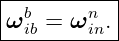
calculations. The central ideal measurement is
which is the angular velocity of the body frame b relative to inertial frame i, resolved in body
coordinates. The quantity required to propagate body attitude relative to a navigation frame n is
instead
The exercises deliberately move through three levels of interpretation:
- the physical sensing mechanism of a gyro;
- the frame-rate bookkeeping required on a rotating Earth;
- numerical propagation of attitude from gyro samples.
Unless otherwise stated, use the WGS-84 Earth rotation rate
Angles used inside trigonometric functions must be converted to radians. The notation follows
INS04 and standard inertial-navigation references [1, 2, 3, 4, 5].
1 Exercises
Exercise 1: A gyro measures rate, not attitude
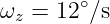
A vehicle begins with yaw
It then rotates at a constant positive yaw rate
for 7.5 s. Assume the navigation frame is inertially fixed for this short example and the motion is a
pure rotation about the common vertical axis.
- Find the accumulated yaw change.
- Find the final yaw.
- If the same rate measurement were obtained but the initial yaw were unknown, could
the final yaw be determined uniquely?
- Explain why this scalar example is simpler than general three-dimensional attitude
propagation.
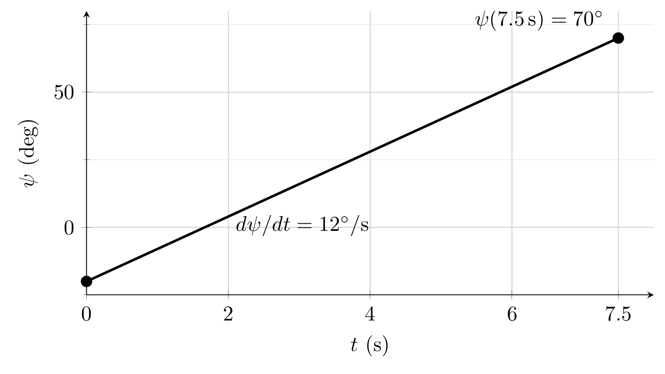
Figure. A constant rate produces a linearly changing yaw only in this special one-axis case.
The gyro supplies the slope, while the initial attitude supplies the integration constant.
Exercise 2: Classical rotor gyro torque and precession
A symmetric rotor has spin-axis moment of inertia
and spins at 18,000 rpm. Its spin-axis angular momentum is perpendicular to a forced precession
rate of 3.00∘∕s.
- Convert the rotor spin rate to radians per second.
- Find the angular-momentum magnitude H = Isωs.
- Convert the precession rate to radians per second.
- Find the torque magnitude required to sustain the precession using
- Explain what part of this calculation gives the rotor gyro its usefulness as an inertial
reference.
Exercise 3: MEMS Coriolis angular-rate sensing
A simplified MEMS gyro drives a proof mass with instantaneous velocity
The sensor rotates with
Use the apparent Coriolis acceleration
The proof mass is 0.50 mg and the sense-axis stiffness is 20.0 N/m.
- Convert the rotation rate to radians per second.
- Find the Coriolis acceleration vector.
- Find the corresponding sense-axis force magnitude.
- If the sense motion is treated quasistatically, estimate the displacement x = F∕k.
- Explain why reversing the drive velocity reverses the Coriolis signal even though the
platform angular rate has not changed.
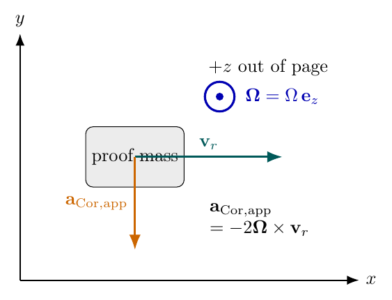
Figure. A MEMS rate gyro converts platform rotation into a transverse Coriolis response
of a driven proof mass. The sign follows the cross product between the platform angular
rate and the drive velocity.
Exercise 4: Earth rate resolved in NED
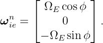
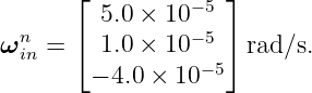
An IMU is stationary relative to the Earth at geodetic latitude
Neglect transport rate. In the local North-East-Down frame, use
- Compute the North, East, and Down components in rad/s.
- Convert those components to degrees per hour.
- Verify that the magnitude remains ΩE.
- How much inertial rotation angle accumulates in one minute if Earth rotation is not
removed?
- Explain why a stationary Earth-fixed gyro does not ideally read zero.
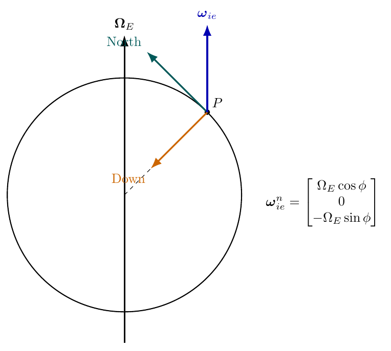
Figure. Earth rate is a physical angular-velocity vector. In local NED coordinates its
North and Down components vary with latitude, while its magnitude remains ΩE.
Exercise 5: What a level body-mounted gyro reads
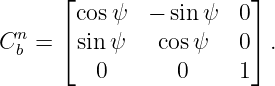
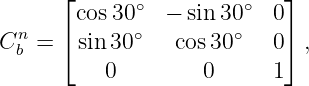
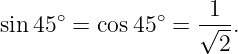
A vehicle is stationary relative to the Earth at latitude 40∘. It is level, but its forward axis is
pointed 30∘ east of north. Thus its yaw is
with zero roll and pitch. Use
- Compute ωien.
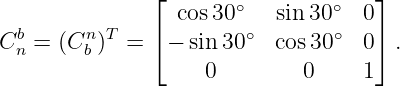
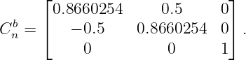
- Form Cnb = (C
bn)T .
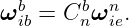
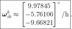
- Compute the ideal gyro triad output
- Convert each body-axis component to degrees per hour.
- Explain why changing heading changes the individual gyro channels but not the angular-rate
magnitude.
Exercise 6: From inertial body rate to body rate relative to navigation
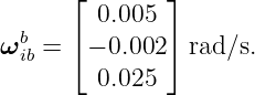
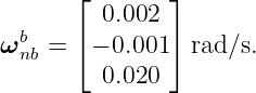
At one instant a strapdown INS has the measured gyro vector
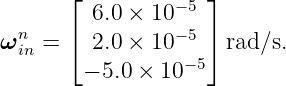
The navigation-frame rate is
The vehicle is level at heading 30∘, with C
bn as defined in Exercise 5.
- Resolve ωinn in body coordinates.
- Compute
- Compare the size of the reference-frame correction to the measured gyro rate.
- Explain why a small correction can still matter when attitude is integrated for a long
time.
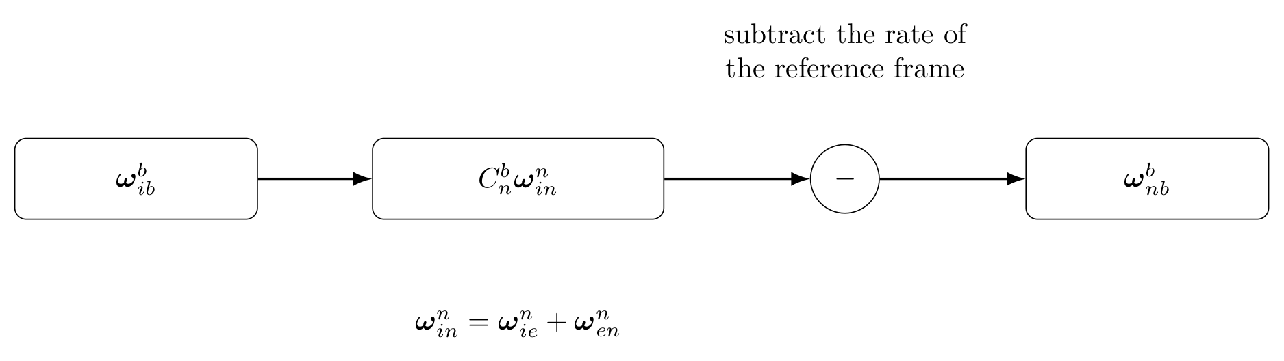
Figure. A gyro measures body rate relative to inertial space. Attitude relative to the
navigation frame requires subtraction of the navigation frame’s own inertial angular rate
after both vectors are expressed in the same coordinates.
Exercise 7: Transport rate of a moving local-level frame
A vehicle moves over the Earth at latitude 45∘ with
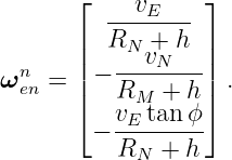
Use
and the NED transport-rate model
- Compute ωenn in rad/s.
- Compute Earth rate ωien at 45∘.
- Form
- Convert the components of all three rate vectors to degrees per hour.
- If the vehicle body is held exactly fixed relative to NED, what ideal angular rate must its
gyro sense relative to inertial space?
Exercise 8: Exact constant-yaw attitude propagation
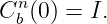
At time t = 0 the body and navigation frames coincide,
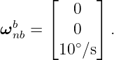
The body rotates relative to the navigation frame at a constant rate
Assume that the relative rate remains exactly along the common Down axis.
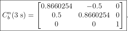
- Find the yaw after 3.0 s.
- Write the exact Cbn(3 s).
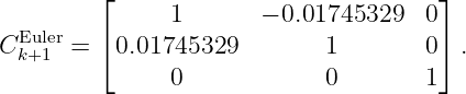
- For a single time step Δt = 0.1 s, form the forward-Euler approximation
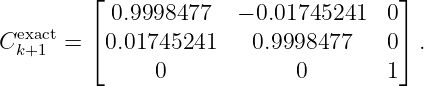
- Compare this one-step approximation with the exact 1∘ finite rotation.
- Evaluate Ck+1T C
k+1 for the Euler step and identify the orthogonality error.
Exercise 9: Verify the full strapdown attitude equation numerically
At one instant,
and the navigation-frame rate is
Suppose the desired body rate relative to navigation is
- Compute the ideal inertial gyro measurement
- Evaluate
- Independently evaluate
- Verify numerically that the two matrices agree.
- Explain what cancellation this demonstrates physically.
Exercise 10: A finite three-dimensional angular increment
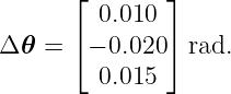
During one IMU sample interval the integrated gyro increment is
- Find the rotation magnitude 𝜃 = |Δ𝜃| in radians and degrees.
- Form S = [Δ𝜃]×.
- Use Rodrigues’ formula
to compute the exact finite-rotation update.
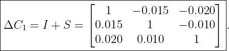
- Form the first-order approximation I + S.
- Compare the matrices and calculate (I + S)T (I + S) − I.
- Explain why finite-rotation propagation is preferable to repeatedly applying I + S without
restoring orthogonality.
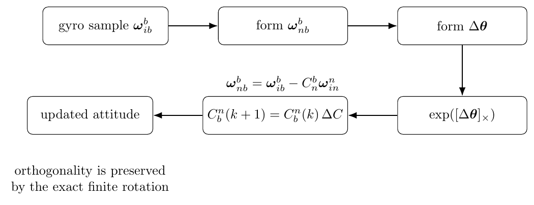
Figure. A practical strapdown attitude step begins with the inertial gyro measurement,
removes reference-frame rotation, integrates a finite angular increment, and updates the
attitude with a proper rotation matrix.
Exercise 11: Constant gyro bias and attitude drift
A stationary platform has a constant unmodeled gyro bias about one axis of
Ignore all other errors and suppose the navigation computer interprets this bias as real angular
motion.
- Convert the bias to rad/s.
- Find the attitude error after 60 s.
- Find the attitude error after 300 s.
- Explain why even a small constant rate error is dangerous in an unaided inertial system.
- Connect the result qualitatively to the INS03 relation between tilt error and false
horizontal acceleration.
2 Worked solutions
Solution 1: A gyro measures rate, not attitude
For this one-axis case,
Since the rate is constant,
| Δψ | = ωzΔt | (27)
|
| = (12∘∕s)(7.5 s) | (28)
|
| = 90∘ . | (29) |
Therefore
| ψf | = ψ0 + Δψ | (30)
|
| = −20∘ + 90∘ | (31)
|
| = 70∘ . | (32) |
If the initial yaw were unknown, the final yaw would also be unknown. The gyro supplies a change
in orientation, not an absolute orientation reference.
The scalar calculation is unusually simple because the rotation axis is fixed. In general
three-dimensional motion, successive rotations do not commute. For example, a 10∘ roll followed by
a 10∘ pitch is not identical to performing the pitch first and the roll second. General strapdown
propagation therefore uses DCMs, quaternions, or another finite-rotation representation rather
than integrating three Euler-angle channels independently.
Solution 2: Classical rotor gyro torque and precession
First convert the rotor speed:
| ωs | = 18,000   | (33)
|
| = 1884.96 rad∕s . | (34) |
The angular momentum is
| H | = Isωs | (35)
|
| = (2.50 × 10⁻⁴)(1884.96) | (36)
|
| = 0.471239 N m s . | (37) |
The precession rate is
| Ωp | = 3.00 | (38)
|
| = 0.0523599 rad∕s . | (39) |
Since Ωp is perpendicular to H,
| τ | = ΩpH | (40)
|
| = (0.0523599)(0.471239) | (41)
|
| = 2.4674 × 10⁻² N m . | (42) |
The key inertial property is conservation of angular momentum. In the absence of torque, the
angular-momentum direction tends to remain fixed in inertial space. A vehicle rotation relative to
that inertial direction therefore creates a measurable mechanical response. Modern strapdown
gyros may use very different hardware, but the quantity being estimated remains an angular rate
relative to inertial space.
Solution 3: MEMS Coriolis angular-rate sensing
Convert the rotation rate:
The drive velocity is along +x and the angular rate is along +z, so
Therefore the apparent Coriolis acceleration is
| aCor,app | = −2Ω × vr | (45)
|
| = −2(2.094395)(0.080) ey | (46)
|
| = −0.335103 ey m∕s2 . | (47) |
The mass is
Hence the force magnitude is
| F | = m|aCor,app| | (49)
|
| = (5.0 × 10⁻⁷)(0.335103) | (50)
|
| = 1.676 × 10⁻⁷ N . | (51) |
With stiffness k = 20.0 N/m, a quasistatic displacement estimate is
| x | =  | (52)
|
| = 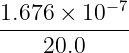 | (53)
|
| = 8.38 × 10⁻⁹ m . | (54) |
This is only several nanometers, which helps explain why MEMS gyros require sensitive mechanical
structures and electronics.
If the drive velocity reverses, vr →−vr. The cross product changes sign:
The rotation has not changed, but the Coriolis response follows the oscillating drive velocity.
Practical MEMS gyros demodulate that sense-axis response against the known drive motion to
recover angular rate.
Solution 4: Earth rate resolved in NED
At ϕ = 45∘,
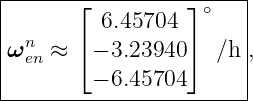
Therefore
| ωien | = 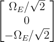 | (57)
|
| = 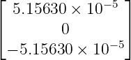 rad∕s . rad∕s . | (58) |
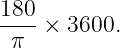
To convert rad/s to degrees per hour, multiply by
Thus
The magnitude is
| |ωien| | =  | (61)
|
| = ΩE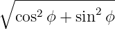 | (62)
|
| = ΩE . | (63) |
In one minute, the inertial rotation angle of the Earth is
| Δ𝜃E | = ΩE(60) | (64)
|
| = 0.00437527 rad | (65)
|
| = 0.250684∘ . | (66) |
A gyro attached to the ground is stationary relative to Earth, but Earth itself rotates relative to
inertial space. Therefore the ideal inertial rate measurement is not zero.
Solution 5: What a level body-mounted gyro reads
At latitude 40∘,
For ψ = 30∘,
Hence
| ωibb | = C
nbω
ien | (69)
|
| = 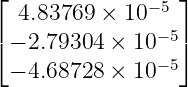 rad∕s . rad∕s . | (70) |
In degrees per hour,
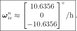
The body components changed because the sensor axes rotated relative to North and East.
However,
because an orthogonal coordinate transformation changes components but not vector
magnitude.
This is a useful static-IMU test. If the IMU orientation is known and the gyro is sufficiently
sensitive, its measured Earth-rate components should agree with the transformed model to within
sensor errors.
Solution 6: From inertial body rate to body rate relative to navigation
Using the same 30∘ level attitude,
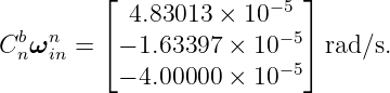
Transform the navigation-frame rate into body coordinates:
| Cnbω
inn | = 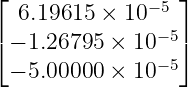 rad∕s . rad∕s . | (74) |
Subtract this from the inertial gyro rate:
| ωnbb | =  − −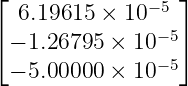 | (75)
|
| = 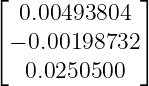 rad∕s . rad∕s . | (76) |
The correction is much smaller than the dominant 0.025 rad/s body rate in this example. However,
attitude is obtained by integration. A reference-frame rate error of only 10−5 to 10−4 rad/s can
accumulate into a visible angle error over minutes or hours. For precision inertial navigation, small
systematic rate terms cannot simply be discarded because they are smaller than the instantaneous
vehicle maneuver rate.
Solution 7: Transport rate of a moving local-level frame
At 45∘, tan ϕ = 1. The transport-rate components are
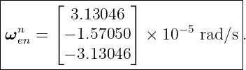
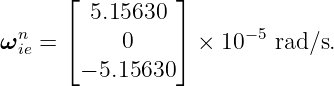
| ωen,Nn | = 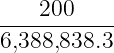 = 3.13046 × 10⁻⁵ rad∕s, = 3.13046 × 10⁻⁵ rad∕s, | (77)
|
| ωen,En | = −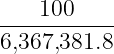 = −1.57050 × 10⁻⁵ rad∕s, = −1.57050 × 10⁻⁵ rad∕s, | (78)
|
| ωen,Dn | = −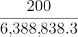 = −3.13046 × 10⁻⁵ rad∕s. = −3.13046 × 10⁻⁵ rad∕s. | (79) |
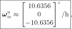
Thus
From Exercise 4,
Therefore
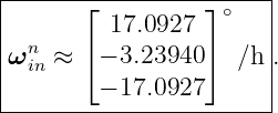
| ωinn | = ω
ien + ω
enn | (82)
|
| = 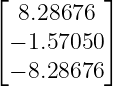 × 10−5 rad∕s . × 10−5 rad∕s . | (83) |
In degrees per hour,
and
If the body is held exactly fixed relative to NED, then
The body must still rotate relative to inertial space at the same angular rate as the local
navigation frame. If body axes are aligned with NED,
The magnitude is approximately
This example shows why the local navigation frame is not merely Earth-fixed. It also rotates
because the vehicle moves over the curved Earth.
Solution 8: Exact constant-yaw attitude propagation
The rate magnitude is
After 3.0 s,
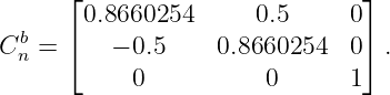
The exact passive body-to-navigation DCM is
For one 0.1 s step, the angular increment is
Starting from Ck = I, forward Euler gives
The exact 1∘ rotation is
The one-step numerical difference is small, but the Euler matrix is not exactly orthogonal:
The diagonal error is second order in the angular increment. Repeated first-order propagation
causes a DCM to drift away from the rotation group unless a finite-rotation update or periodic
orthogonality restoration is used.
Solution 9: Verify the full strapdown attitude equation numerically
For the given 30∘ yaw,
Transform the navigation-frame rate to body coordinates:
Therefore the ideal inertial gyro measurement is
| ωibb | = ω
nbb + C
nbω
inn | (99)
|
| = 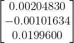 rad∕s . rad∕s . | (100) |
Substitution into the full attitude equation gives
Now evaluate the relative-rate form directly:
It produces the same matrix to numerical roundoff. The identity follows algebraically
from
and the cross-product transformation identity
When multiplied by Cbn, the contribution of the navigation-frame rate in the gyro measurement
cancels the explicit
term. What remains is exactly the rotation of body relative to navigation. This is the physical
meaning of the full strapdown attitude equation.
Solution 10: A finite three-dimensional angular increment
The increment magnitude is
| 𝜃 | =  | (106)
|
| = 0.0269258 rad | (107)
|
| = 1.54274∘ . | (108) |
The skew-symmetric matrix is
Rodrigues’ formula gives
The first-order approximation is
Its orthogonality defect is
The Frobenius norm of this defect is approximately
The exact Rodrigues update is a member of SO(3), so it preserves orthogonality and determinant
+1 apart from numerical roundoff. The linear approximation is useful in derivations and
error-state models, but repeated attitude propagation should use a proper finite-rotation
update.
This example also shows why a three-component angular increment is not simply three
independent Euler-angle increments. The vector Δ𝜃 defines one finite rotation through
the exponential map. The coupling between axes appears in the S2 and higher-order
terms.
Solution 11: Constant gyro bias and attitude drift
Convert the bias to radians per second:
| bg | = 0.020 | (114)
|
| = 3.49066 × 10⁻⁴ rad∕s . | (115) |
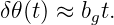
For a constant unmodeled bias, the small-angle attitude error initially grows approximately
as
After 60 s,
| δ𝜃(60) | = (0.020∘∕s)(60 s) | (117)
|
| = 1.20∘ . | (118) |
After 300 s,
| δ𝜃(300) | = (0.020∘∕s)(300 s) | (119)
|
| = 6.00∘ . | (120) |
This is dangerous because the attitude solution is used to rotate accelerometer specific force into
the navigation frame. A tilt error causes part of the large gravity-related specific-force vector to
leak into a horizontal channel. For a small horizontal tilt error,
Therefore a gyro rate bias can become an attitude error, then a false horizontal acceleration, then
velocity and position errors after further integration. INS19 will derive this error chain in
detail.
3 What these exercises establish
The worked examples above establish several habits that are central to strapdown navigation:
- A gyro measures angular rate, not attitude. An initial attitude and a
rotation-propagation law are still required.
- Mechanical rotor gyros, MEMS vibrating-mass gyros, and optical gyros use different
physics but target an angular rate relative to inertial space.
- A stationary Earth-fixed gyro can have a nonzero ideal output because the Earth
rotates relative to inertial space.
- Earth rate must be resolved in the sensor coordinates before it can be compared with
body-axis gyro measurements.
- A local navigation frame rotates because of both Earth rotation and vehicle motion
over the curved Earth.
- The attitude-propagation rate is ωnbb, not directly the measured ω
ibb.
- The full attitude equation and the relative-rate form are mathematically equivalent
when frame-rate transformations are handled consistently.
- First-order DCM updates are useful approximations but do not preserve orthogonality
exactly.
- Finite angular increments should be propagated with a proper rotation update such as
Rodrigues’ formula or an equivalent quaternion update.
- Small systematic gyro errors accumulate in attitude and can couple into large
translational navigation errors.
These results prepare the reader for INS05, where the gravity and effective-gravity models required
by the translational mechanization will be developed in detail. They also prepare the mathematical
ground for INS08, where quaternion attitude propagation will be derived from the same
angular-rate measurements.
References
[1] D. H. Titterton and J. L. Weston, Strapdown Inertial Navigation Technology, 2nd
ed., IET, 2004.
[2] P. D. Groves, Principles of GNSS, Inertial, and Multisensor Integrated Navigation
Systems, 2nd ed., Artech House, 2013.
[3] C. Jekeli, Inertial Navigation Systems with Geodetic Applications, Walter de Gruyter,
2001.
[4] A. Lawrence, Modern Inertial Technology: Navigation, Guidance, and Control, 2nd
ed., Springer, 1998.
[5] P. G. Savage, “Strapdown Inertial Navigation Integration Algorithm Design Part 1:
Attitude Algorithms,” Journal of Guidance, Control, and Dynamics, vol. 21, no. 1, pp.
19–28, 1998.
[6] J. E. Bortz, “A New Mathematical Formulation for Strapdown Inertial Navigation,”
IEEE Transactions on Aerospace and Electronic Systems, vol. AES-7, no. 1, pp. 61–66,
1971.

![[parent]](https://images.physicslibrary.org/images/uparrow.png)















![( b )
Ck+1 ≈ Ck I + [ωnb]×Δt .](https://images.physicslibrary.org/cache/objects/1351/make4ht/StrapdownInertialNavigationExamplesGyroscopeAngularRateSensingAndAttitudePropagation24x.png)

![dCn
---b-= Cnb [ωbib]× − [ωnin]×Cnb .
dt](https://images.physicslibrary.org/cache/objects/1351/make4ht/StrapdownInertialNavigationExamplesGyroscopeAngularRateSensingAndAttitudePropagation29x.png)
![n b
Cb [ω nb]×.](https://images.physicslibrary.org/cache/objects/1351/make4ht/StrapdownInertialNavigationExamplesGyroscopeAngularRateSensingAndAttitudePropagation30x.png)
















![Cnb [ωbnb]×.](https://images.physicslibrary.org/cache/objects/1351/make4ht/StrapdownInertialNavigationExamplesGyroscopeAngularRateSensingAndAttitudePropagation85x.png)

![b n b n n
[C nω in]× = C n[ωin]×C b .](https://images.physicslibrary.org/cache/objects/1351/make4ht/StrapdownInertialNavigationExamplesGyroscopeAngularRateSensingAndAttitudePropagation87x.png)
![− [ωnin]×Cnb](https://images.physicslibrary.org/cache/objects/1351/make4ht/StrapdownInertialNavigationExamplesGyroscopeAngularRateSensingAndAttitudePropagation88x.png)
![⌊ ⌋
0 − 0.015 − 0.020
S = [Δ 𝜃]× = ⌈0.015 0 − 0.010⌉ .
0.020 0.010 0](https://images.physicslibrary.org/cache/objects/1351/make4ht/StrapdownInertialNavigationExamplesGyroscopeAngularRateSensingAndAttitudePropagation90x.png)