Strapdown Inertial Navigation: Gravity, Gravitation, and the Rotating Earth
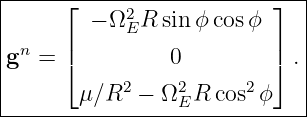
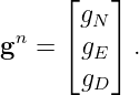
Gravity enters inertial navigation in a deceptively simple-looking place. Once accelerometer
specific force has been transformed into the navigation frame, the mechanization adds a
gravity vector before integrating velocity. In local north-east-down coordinates one often
sees
The symbol gn can make gravity look like a single external correction that is simply inserted into
the equations. Physically, however, several ideas are hiding inside it.
Earth’s mass distribution produces gravitation. Earth also rotates. A navigation equation written
in a frame fixed to that rotating Earth contains a centrifugal contribution. The vector
conventionally called local gravity combines these effects, with smaller corrections added when
greater geophysical fidelity is required [1, 2, 3].
This entry develops that structure from Newtonian gravitation and the rotating-frame derivative
derived in INS02. The goal is not merely to quote a gravity formula. The goal is to understand why
the form of the strapdown velocity equation depends on exactly what quantity the gravity model
represents.
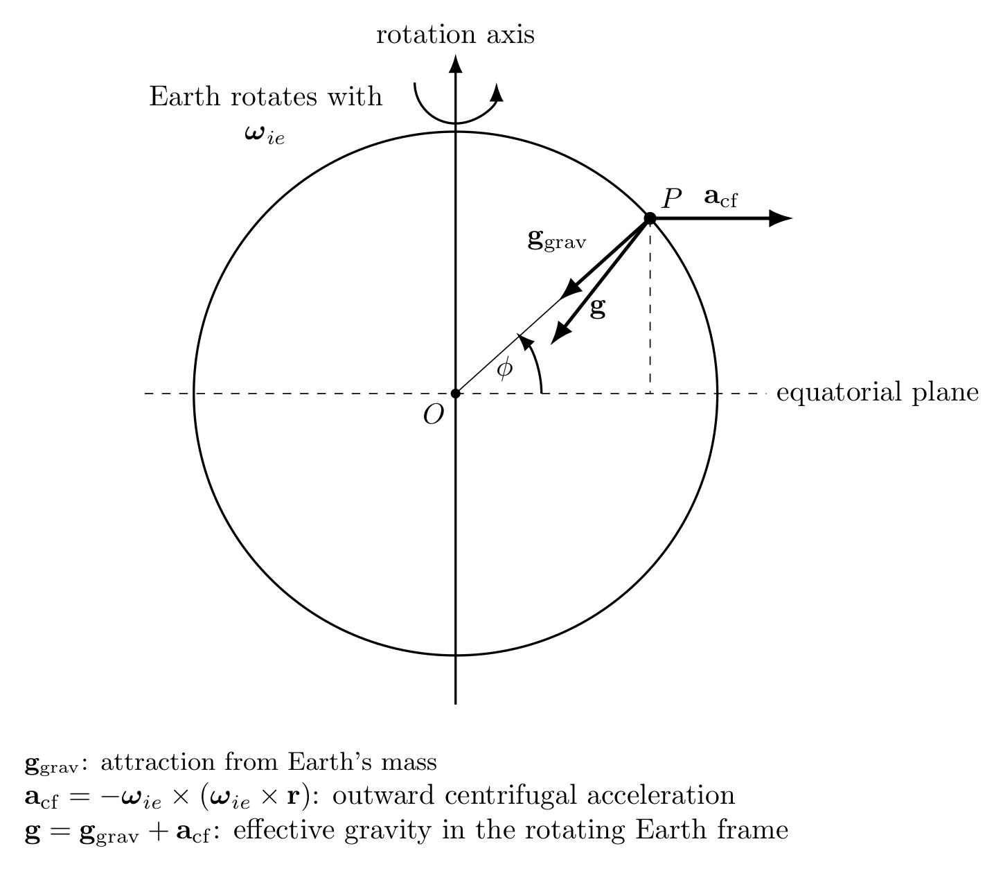
Figure. Gravitation points approximately toward Earth’s mass center. The centrifugal
acceleration associated with an Earth-fixed rotating frame points away from the rotation
axis. Their vector sum is the effective gravity used by an Earth-fixed navigation
mechanization.
1 Learning objectives
After completing this entry, the reader should be able to:
- distinguish gravitation from effective gravity;
- derive the point-mass gravitational acceleration from a scalar potential;
- derive the centripetal acceleration of a point fixed to the rotating Earth;
- identify the outward centrifugal term that appears when Newton’s law is rewritten in
an Earth-fixed rotating frame;
- define effective gravity as the combination of gravitation and centrifugal acceleration;
- explain why an accelerometer at rest on Earth measures approximately the negative
of effective gravity;
- derive the latitude dependence of the centrifugal contribution on a spherical Earth;
- explain why an oblate rotating ellipsoid is a better reference model than a nonrotating
sphere;
- use the WGS-84 Somigliana normal-gravity formula;
- estimate the first-order change of gravity with altitude;
- derive the ECEF strapdown velocity equation first with an explicit centrifugal term
and then with effective gravity absorbed into ge;
- interpret the corresponding local NED velocity equation;
- identify gravity-model errors that can produce velocity and position drift.
2 Terminology: gravitation is not exactly the same as gravity
The words gravity and gravitation are often used interchangeably in introductory mechanics. In
navigation and geodesy it is useful to distinguish them.
In this entry we use the following convention.
and
For the simplest rotating-Earth model,
The second term is outward from Earth’s rotation axis because
is inward toward that axis. Therefore its negative is the centrifugal acceleration of the rotating
description.
Some texts use slightly different terminology. For example, the word “gravity” may already imply a
normal-gravity model on a rotating ellipsoid. The equations are unambiguous as long as the
quantity being modeled is stated explicitly.
3 Newtonian gravitation from a potential
Start with the simplest Earth model: a spherically symmetric body of mass M. Outside such a
body, Newton’s shell theorem allows The Gravitational Field to be treated as if all mass were
concentrated at Earth’s center.
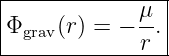
Let
where G is the Newtonian gravitational constant and M is Earth’s mass. The gravitational
potential per unit mass is
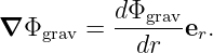
The gravitational acceleration is the negative gradient of the potential:
Because the potential depends only on the radial distance r,
Now
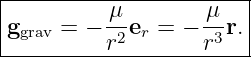
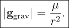
Therefore
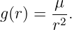
The acceleration is directed toward Earth’s center and has magnitude
This point-mass result is the first gravity model in the navigation hierarchy. It is simple, physically
transparent, and useful for deriving error trends. It is not accurate enough to represent the real
rotating, oblate Earth at high precision.
4 The gravity gradient in the spherical model
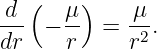
The same equation immediately explains why gravity decreases with height. Let
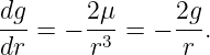
Differentiate with respect to r:
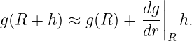
For a small altitude increment h relative to an Earth radius R,
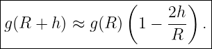
Hence
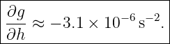
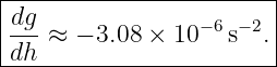
Taking R ≈ 6.37 × 10⁶ m and g ≈ 9.81 m∕s2 gives a vertical gradient near the surface of
about
Thus a 1000 m increase in height reduces gravity by roughly
in this first-order spherical estimate.
5 A point fixed to Earth is not fixed in inertial space
Now include Earth’s rotation. Let the Earth-fixed frame e rotate relative to inertial frame i with
angular velocity
Consider a point whose Earth-fixed coordinates are constant. It is stationary in ECEF
coordinates, but it moves in a circle around Earth’s rotation axis when viewed from inertial
space.
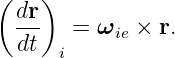
From the transport theorem developed in INS02, with Earth rotation treated as constant,
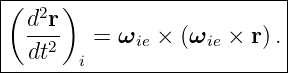
Differentiating again in inertial space gives
This vector points inward toward the rotation axis. It is the centripetal acceleration required for
the point to remain fixed on the rotating Earth.
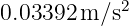
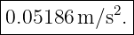
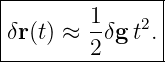
At the equator, its magnitude is approximately
Using
and
we obtain
This is small compared with 9.8 m∕s2, but it is far too large to ignore in inertial navigation.
6 Surface force balance and what the accelerometer senses
The distinction between gravitation and effective gravity can be seen directly from Newton’s
second law for an IMU resting on Earth.
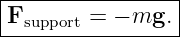
Suppose the non-gravitational support force exerted by the vehicle structure on the IMU is
Fsupport. In inertial space,
For an Earth-fixed point,
Therefore
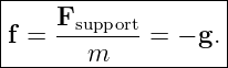
Define effective gravity by
Then
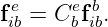
Since an ideal accelerometer measures non-gravitational force per unit mass,
This result generalizes the INS03 statement that a supported accelerometer reads approximately
1g. On a rotating Earth, the supported accelerometer is reacting to effective gravity, not to
gravitation alone.
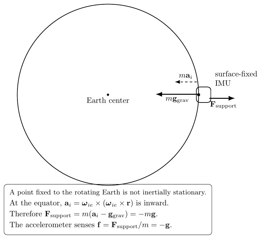
Figure. A surface-fixed IMU has inward centripetal acceleration in inertial space.
Gravitation and the support force therefore do not cancel exactly. Their difference supplies
the required centripetal acceleration. The accelerometer measures the support force per
unit mass, which is the negative of effective gravity.
7 The centrifugal acceleration in the rotating Earth frame
INS02 derived the general relation between inertial acceleration and acceleration observed in a
rotating frame. For the Earth-fixed frame, assuming constant Earth rotation,
Newton’s law in inertial space is
Substitute the first equation into the second and solve for the Earth-fixed acceleration:
The last term is the outward centrifugal acceleration in the Earth-fixed equation:
This is the same physical geometry discussed in INS02. The sign changes because we have
rearranged the inertial acceleration relation to solve for acceleration measured in the rotating
frame.
The effective-gravity definition
therefore gives
This compact form is the key reason Normal gravity models are convenient in Earth-fixed
navigation equations: the centrifugal contribution has already been absorbed into g.
8 Centrifugal acceleration versus latitude on a spherical Earth
The latitude dependence can be derived geometrically. Consider a spherical Earth of radius R. At
latitude ϕ, the perpendicular distance from the rotation axis is
The magnitude of the centrifugal acceleration is
The vector points horizontally away from the rotation axis, not directly away from Earth’s center
except at the equator.
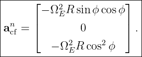
Resolve this vector into local north and down components on a spherical Earth. The result
is
The north component is negative in the northern hemisphere, so the centrifugal contribution points
slightly southward toward the equator. The down component is negative because centrifugal
acceleration acts upward relative to the local radial direction.
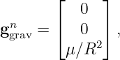
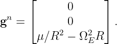
If the point-mass gravitation vector is purely down,
then the effective gravity in the spherical model is
Two useful limiting cases follow immediately.
At the equator, ϕ = 0:
At the pole, ϕ = 90∘:
Thus rotation reduces apparent gravity most strongly at the equator and not at all at the rotation
axis.
9 Why a spherical Earth is still not enough
Earth is not spherical. Its rotation and long-term hydrostatic structure produce an oblate shape,
with an equatorial radius larger than the polar radius. This affects navigation gravity in two
coupled ways.
First, the distance from Earth’s center depends on latitude. Since gravitational attraction
scales roughly as 1∕r2, the shorter polar radius tends to increase gravitation near the
poles.
Second, the centrifugal acceleration itself depends on distance from the rotation axis and vanishes
at the poles.
The observed increase in normal gravity from equator to pole therefore contains both rotational
and geometric effects. The equatorial centrifugal acceleration of approximately
is substantial, but it is not the whole reason normal gravity differs between equator and
pole.
A convenient navigation reference model is therefore a rotating oblate ellipsoid whose gravity field
is chosen consistently with its shape and angular velocity. WGS-84 provides such a reference
system [5, 2].
10 WGS-84 reference ellipsoid
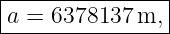
Several WGS-84 parameters are central to inertial navigation and geodesy. The semi-major axis
is
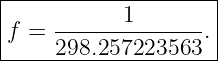
and the flattening is
The first eccentricity squared is
The conventional Earth rotation rate is
WGS-84 also specifies the geocentric gravitational constant
These parameters are not independent decoration. The ellipsoid geometry, rotation, and reference
gravity field are designed to work together.
11 Normal gravity on the reference ellipsoid
For many strapdown applications, the gravity vector is approximated by normal gravity, the
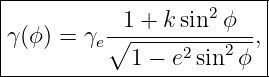
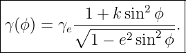
gravity field of the chosen rotating reference ellipsoid. At the ellipsoid surface, Somigliana’s formula
can be written
where ϕ is geodetic latitude, γe is normal gravity at the equator, and k is the Somigliana constant
[4, 5].
For WGS-84, useful values are
At selected latitudes this gives approximately
| Geodetic latitude | Normal gravity γ (m/s2) |
|
|
| 0∘ | 9.7803253 |
| 30∘ | 9.7932473 |
| 45∘ | 9.8061978 |
| 60∘ | 9.8191770 |
| 90∘ | 9.8321849 |
The pole-to-equator difference is about
That is more than five thousandths of g, which is enormous on the scale of inertial-navigation
errors.
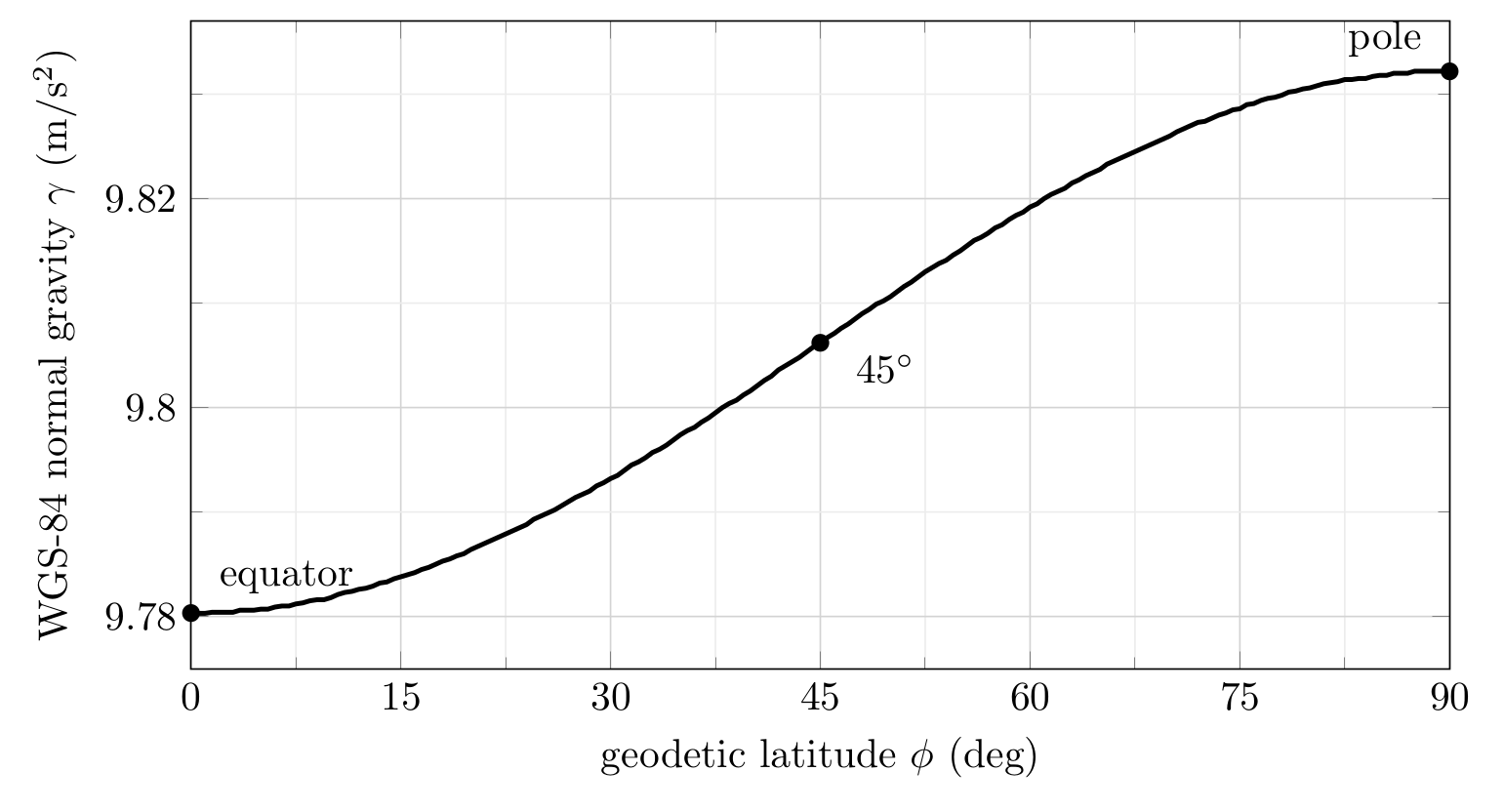
Figure. WGS-84 normal gravity increases from the equator to the poles. The trend
contains both the effect of Earth rotation and the oblate reference geometry.
12 Normal gravity above the ellipsoid
A navigation system rarely remains exactly on the reference ellipsoid. Gravity must therefore be
adjusted for height.
The simplest physical approximation comes from the spherical result already derived:
More accurate normal-gravity formulas include latitude-dependent height terms and
ellipsoidal geometry. Groves and Jekeli provide forms suitable for navigation implementations
[2, 3].
For conceptual work near Earth’s surface, it is useful to remember the approximate free-air
gradient
A 1 km altitude error therefore corresponds to a gravity-magnitude error of order
if height dependence is ignored entirely.
13 Normal gravity is not the complete real gravity field
The WGS-84 normal field is deliberately smooth. The actual gravity field differs because Earth’s
mass distribution is irregular.
Important deviations include:
- large-scale spherical-harmonic structure of the terrestrial gravity field;
- regional gravity anomalies caused by variations in crust and mantle density;
- mountains, ocean trenches, and local terrain;
- deflection of the vertical, where the true gravity direction differs slightly from the
reference-ellipsoid normal;
- tidal effects from the Moon and Sun;
- temporal redistribution of atmosphere, oceans, groundwater, and ice.
The required gravity fidelity depends on the navigation problem. For short-duration or lower-grade
inertial systems, a normal-gravity model may be more than adequate. High-accuracy inertial
navigation, inertial surveying, submarine navigation, and gravimetry can require substantially
more detailed models.
The important architectural idea is that the mechanization needs a gravity vector appropriate to
the chosen navigation frame and fidelity level. The source of that vector can evolve without
changing the fundamental strapdown equations.

Figure. A useful hierarchy of gravity models. Point-mass gravitation exposes the physics.
Rotating spherical and ellipsoidal models add the dominant Earth effects. High-accuracy
systems can add gravity harmonics, anomalies, terrain, and time-dependent corrections.
14 Gravity in local NED coordinates
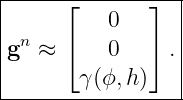
For a local north-east-down frame,
In the simplest normal-gravity mechanization, the local vertical is chosen so that the reference
normal gravity points along the down axis. Then
This sign is easy to mishandle. NED uses positive down, so gravity has a positive third
component.
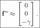
A level stationary accelerometer, by contrast, measures the support specific force
The two vectors cancel in the translational mechanization of a stationary vehicle.
If a higher-fidelity gravity model predicts horizontal gravity components, then gN and gE need not
be exactly zero. Those components can represent deflection of the vertical relative to the reference
ellipsoid.
15 Deriving the ECEF strapdown velocity equation
We can now connect the gravity physics directly to the navigation equations.
Let
be the velocity of body b relative to Earth e, resolved in Earth-fixed coordinates. The
accelerometers provide
Transforming specific force into ECEF gives
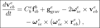
Start with Newton’s law in an inertial frame:
Using the rotating-frame acceleration relation from INS02 and resolving the result in ECEF
gives
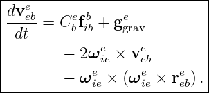
This form displays all the physics explicitly.
Now define effective Earth-fixed gravity as
The velocity equation becomes
Nothing has disappeared physically. The centrifugal term has been absorbed into the definition of
ge.
16 Deriving the local NED velocity equation
The navigation frame n is not fixed to ECEF. As the vehicle moves over Earth’s curved surface,
the local NED frame rotates relative to ECEF with transport rate
The derivative of velocity components in NED therefore differs from the ECEF derivative by
another transport term. Applying the transport theorem gives the local-level velocity
equation
Each term now has a clear origin.
is the non-gravitational specific force measured by the accelerometers and rotated into
NED.
is effective gravity, usually supplied by a normal-gravity or higher-fidelity model.
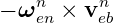
is the Coriolis contribution associated with Earth rotation.
appears because the local NED frame itself rotates as the vehicle moves over Earth.
The centrifugal acceleration due to Earth rotation is not written separately because it is already
part of gn.
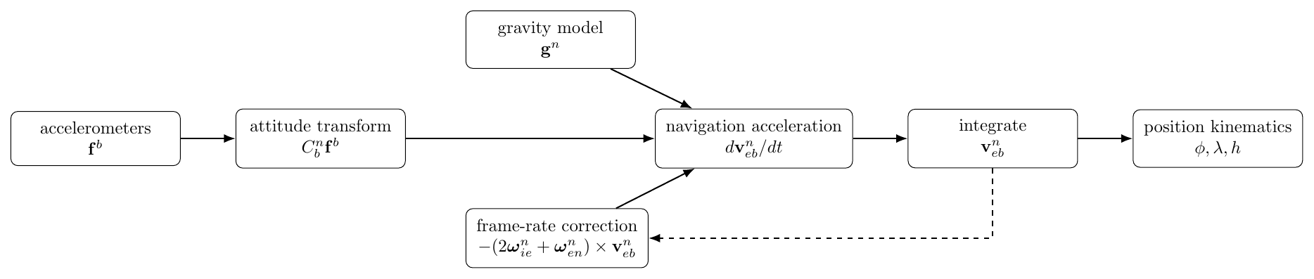
Figure. The translational mechanization combines transformed accelerometer specific
force, the gravity model, and rotating-frame corrections to obtain navigation-frame
acceleration. Velocity and position follow by integration and position kinematics.
17 A stationary NED sanity check
Consider a level IMU fixed to Earth. Its Earth-relative velocity is zero:
Its navigation acceleration must also be zero:
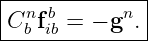
The velocity equation therefore reduces to
Hence
For a level body aligned with NED,
so
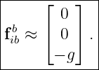
This is an extremely valuable software test. A static mechanization should not accelerate merely
because the accelerometers report approximately −g along the body down axis. The transformed
specific force and gravity model should cancel.
18 What happens if centrifugal acceleration is counted twice?
A common conceptual implementation error is to use a gravity model that already includes
centrifugal acceleration and then also subtract the explicit centrifugal term in the ECEF velocity
equation.
Suppose ge is effective gravity:
The correct ECEF equation is
If an implementation additionally subtracts
then the centrifugal effect has been applied twice.
At the equator the erroneous acceleration magnitude is of order
which would produce a velocity error of roughly
after only one minute if it were allowed to integrate uncompensated.
The cure is not a sign tweak. The cure is to state clearly whether the gravity function returns
gravitation alone or effective gravity.
19 Gravity-model error and navigation drift
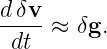
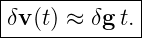
Suppose the gravity model has a small constant error
If all other quantities are ideal, the resulting velocity error initially satisfies
Therefore
Integrating once more,
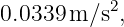
For example, a constant vertical gravity error of
would produce, in this simple uncoupled estimate, a velocity error after 60 s of
and a position error of
The full INS error dynamics are more complicated because attitude, velocity, position,
Earth curvature, and gravity are coupled. INS19 will derive those coupled dynamics.
The simple estimate already shows why gravity-model errors integrate into navigation
errors.
20 A useful implementation hierarchy
For an educational or engineering strapdown implementation, the gravity model can be developed
in stages.
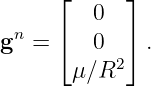
- Point mass. Use −μr∕r3. This is ideal for verifying frame transformations and signs.
- Rotating spherical Earth. Add the centrifugal contribution explicitly or absorb it
into an effective-gravity function.
- WGS-84 normal gravity. Use geodetic latitude and height with a rotating reference
ellipsoid. This is a practical baseline for many navigation systems.
- Higher-fidelity gravity. Add spherical harmonics, gravity anomalies, deflection of
the vertical, terrain, or time-varying corrections when the mission requires them.
At every stage, the interface should make the physical meaning of the returned vector
explicit.
A function named simply
gravity(position)
can be ambiguous. Internally, it is often safer to distinguish concepts such as
gravitation_ecef(position)
effective_gravity_ecef(position)
normal_gravity_ned(latitude, height)
so the mechanization cannot accidentally count centrifugal acceleration twice.
21 Relation to the attitude solution
Gravity also plays a second role in inertial navigation. It is not only a translational acceleration
model. During static or quasi-static alignment, the accelerometers provide the direction opposite
local gravity:
This makes gravity a reference vector for estimating roll and pitch. However, gravity alone cannot
determine yaw because rotating the body about the gravity vector leaves the measured vector
unchanged.
INS09 will combine gravity with Earth rotation to derive coarse alignment and gyrocompassing.
The present lesson provides the physical gravity vector needed for that derivation.
22 Where the series goes next
INS06 will develop the Earth-fixed and local navigation frames in greater detail. It will derive
Earth rate resolved in NED and begin the geometry behind transport rate.
The subsequent sequence will then use the pieces established so far:
- INS07 will derive attitude kinematics from gyro measurements;
- INS08 will develop quaternion propagation;
- INS09 will combine gravity and Earth rate for initial alignment;
- INS10 will return to translational dynamics in an inertial frame;
- INS11 will derive the complete Earth-fixed rotating-frame navigation equations;
- INS12 will assemble an ECEF strapdown mechanization;
- INS13 and INS14 will derive local-level transport rate and ellipsoidal position
kinematics;
- INS15 will assemble the complete NED strapdown mechanization.
23 Summary
Newtonian gravitation for a spherical Earth begins with
Because Earth rotates, a point fixed to Earth has inertial centripetal acceleration
When Newton’s law is written in an Earth-fixed frame, the corresponding outward centrifugal
acceleration is
Effective gravity is therefore
On the WGS-84 reference ellipsoid, normal gravity varies with geodetic latitude. Somigliana’s
formula gives
The ECEF velocity equation can be written with gravitation and centrifugal acceleration shown
separately,
or more compactly using effective gravity,
In local NED coordinates the corresponding navigation equation is
The essential implementation question is therefore not merely “what is g?” It is “what physical
effects are already contained in the gravity vector supplied to this particular navigation
equation?”
References
[1] David H. Titterton and John L. Weston, Strapdown Inertial Navigation Technology,
2nd ed., Institution of Electrical Engineers, 2004.
[2] Paul D. Groves, Principles of GNSS, Inertial, and Multisensor Integrated Navigation
Systems, 2nd ed., Artech House, 2013.
[3] Christopher Jekeli, Inertial Navigation Systems with Geodetic Applications, Walter
de Gruyter, 2001.
[4] Helmut Moritz, “Geodetic Reference System 1980,” Bulletin Geodesique, vol. 54, pp.
395–405, 1980.
[5] National Geospatial-Intelligence Agency, Department of Defense World Geodetic
System 1984: Its Definition and Relationships with Local Geodetic Systems,
NGA.STND.0036, Version 1.0.0, 2014.
[6] Weikko A. Heiskanen and Helmut Moritz, Physical Geodesy, W. H. Freeman, 1967.
















![F = m [ω × (ω × r) − g ].
support ie ie grav](https://images.physicslibrary.org/cache/objects/1352/make4ht/StrapdownInertialNavigationGravityGravitationAndTheRotatingEarth27x.png)