Strapdown Navigation: Time Derivatives in Rotating Frames
A vector can have the same geometric meaning while its numerical components change simply
because the coordinate basis is rotating. This fact is the source of some of the most recognizable
terms in inertial navigation: Earth-rate corrections, transport rate, Coriolis acceleration, and the
distinction between inertial and Earth-fixed dynamics.
INS01 developed coordinate transformations at one instant of time. INS02 asks the next
question:
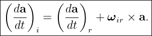
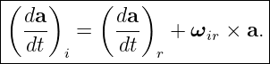
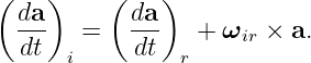
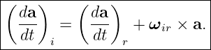
The answer is the transport theorem. For a physical vector a observed from an inertial frame i and
a rotating frame r,
Here ωir is the angular velocity of frame r relative to frame i. This equation will be derived from
the motion of the basis vectors rather than quoted as a rule.
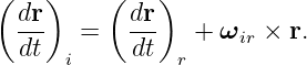
Applying the theorem twice to position leads to
for frames sharing an origin. Coriolis, Euler, and rotational centripetal terms therefore arise from
ordinary differentiation in a moving basis; they are not arbitrary corrections added to Newton’s
laws.
This result is central to strapdown navigation. Earth-fixed coordinates rotate relative to inertial
space, local-level coordinates rotate as a vehicle moves over the Earth, and the body frame rotates
with the vehicle. The navigation equations are built by applying this same geometric theorem
repeatedly [1, 2, 3].
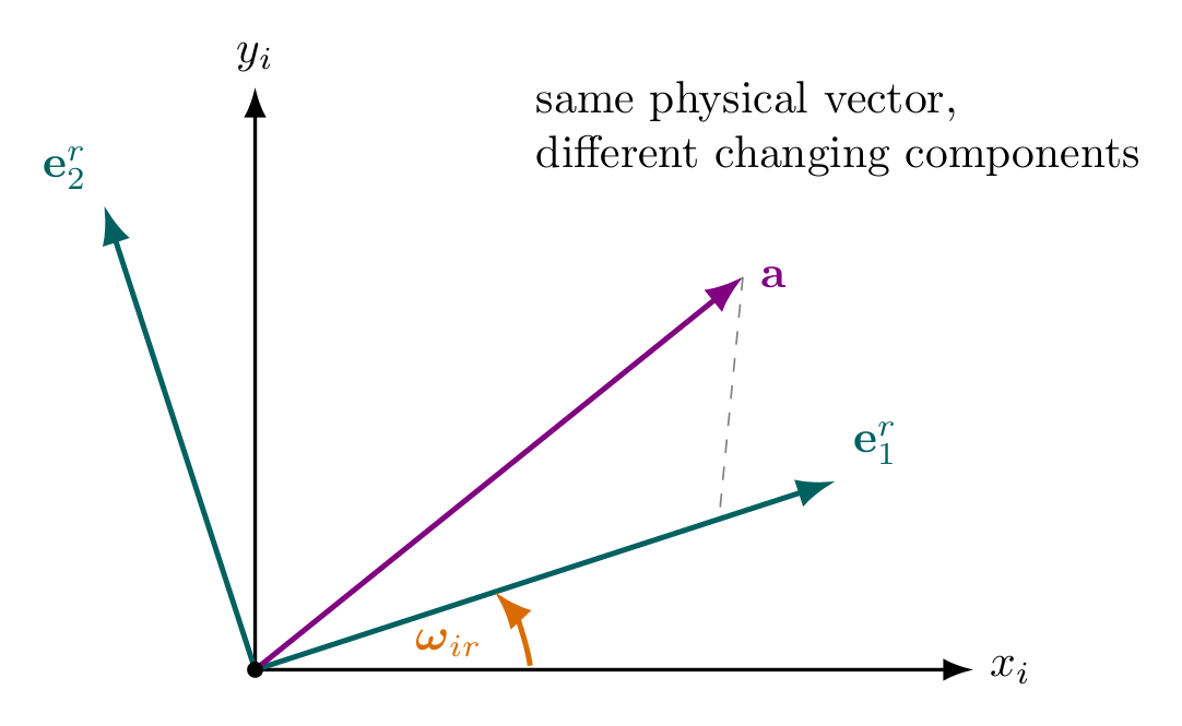
Figure. An inertial basis i and a rotating basis r. Even when a physical vector is
unchanged, its components in the rotating basis can vary because the basis vectors
themselves rotate with angular velocity ωir.
1 Learning objectives
After completing this entry, the reader should be able to:
- distinguish a time derivative of a physical vector from the time derivative of its
coordinate components;
- derive the first-order change of a vector under an infinitesimal rotation;
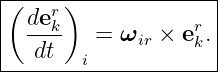
- prove that a rotating unit basis vector satisfies
- derive the transport theorem from a rotating orthonormal basis;
- write the transport theorem in skew-matrix and coordinate form;
- derive the relationship between relative and inertial velocity;
- derive the complete rotating-frame acceleration relationship;
- identify Coriolis, Euler, and rotational centripetal terms and distinguish them from the
apparent centrifugal term;
- extend the result to a rotating frame whose origin also translates;
- explain why a point fixed in a rotating frame can have nonzero inertial velocity and
acceleration;
- explain why a vector fixed in inertial space can have changing coordinates in a rotating
frame;
- connect the transport theorem to DCM time derivatives and later strapdown attitude
kinematics;
- identify where Earth rotation and navigation-frame transport will enter the inertial-navigation
equations.
2 Why an ordinary derivative is not enough
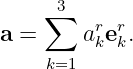
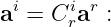
Suppose a physical vector a is expressed in the rotating basis
Then
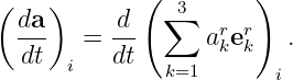
Differentiate this expression as seen from inertial frame i:
Applying the product rule gives
There are therefore two distinct causes of change:
- the scalar components akr can change;
- the basis vectors ekr can rotate.
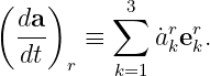
The first term is what an observer attached to frame r calls the derivative of a. The second term is
the contribution caused purely by the rotating basis.
This distinction is the central idea of the article.
3 Infinitesimal rotation of a vector
Consider a vector e attached to a rigid rotating frame. Over a small time interval Δt, suppose the
frame undergoes the small rotation vector
The direction of Δ𝜃 is the instantaneous rotation axis and its magnitude is the small rotation
angle in radians.
To first order, the change of any vector rigidly attached to the rotating frame is
The direction follows from the right-hand rule. The cross product is perpendicular to both the
rotation axis and the original vector, which is exactly the tangent direction in which the vector tip
moves on the unit sphere.
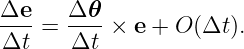
Divide by Δt:
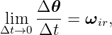
In the limit Δt → 0,
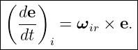
so
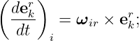
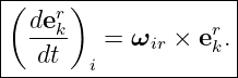
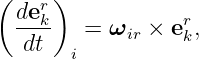
Applied to every rotating basis vector,
This basis-vector derivative is the geometric engine behind the transport theorem.
4 Derivation of the transport theorem
Return to
The inertial derivative is
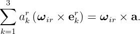
Using the rotating-basis derivative,
Because the cross product is linear,
Since the sum reconstructs the physical vector,
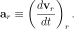
Define
Therefore
This is the transport theorem, also called the rotating-frame derivative theorem.
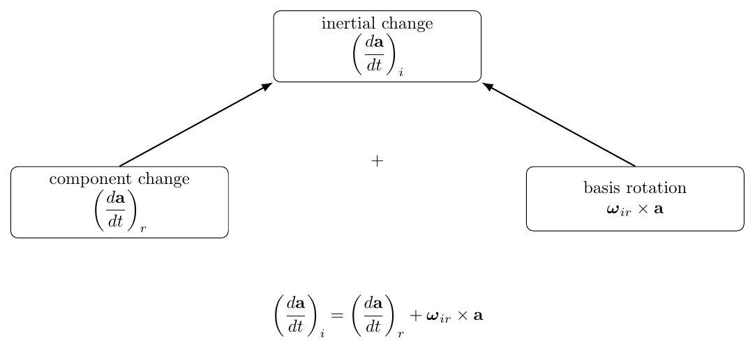
Figure. The inertial change of a vector contains two pieces: change of its components
relative to the rotating frame and change caused by rotation of the basis itself.
5 Coordinate form of the transport theorem
INS01 introduced the skew-symmetric cross-product matrix
If every quantity is resolved in frame r, then the transport theorem becomes
The dot on ar means the derivative of the coordinate column while the r basis is regarded as fixed.
The second term restores the motion of that basis relative to inertial space.
This equation is often what actually appears in navigation software, but its meaning is clearest
only after the geometric derivation above.
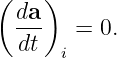
6 A diagnostic example: a vector fixed in inertial space
Suppose a is physically constant in inertial space. Then
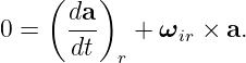
The transport theorem gives
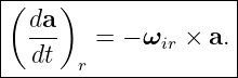
Hence
So an inertially fixed vector appears to rotate backward when observed from the rotating
frame.
This is exactly what should happen. If a turntable rotates counterclockwise beneath an
inertially fixed arrow, an observer standing on the turntable sees that arrow rotate
clockwise.
The minus sign is therefore physical, not merely algebraic.
7 Velocity from the transport theorem
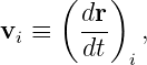
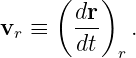
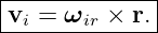
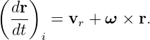
Let r be the position vector of a point measured from the common origin of frames i and r. Apply
the transport theorem to r:
Define
and
Then
This has a direct physical interpretation:
- vr is motion relative to the rotating frame;
- ωir × r is the velocity caused solely by carrying the point around with the rotating
coordinates.
7.1 Point fixed to a turntable
If the point is bolted to the rotating frame,
Nevertheless,
Thus “at rest in the rotating frame” does not mean “at rest inertially.”
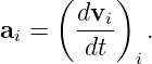
8 Acceleration: applying the theorem a second time
Differentiate the inertial velocity
where, for compactness in this section,
The inertial acceleration is
Therefore
Treat the two terms separately.
8.1 Derivative of the relative velocity
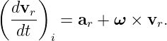
Apply the transport theorem to vr:
Define
Then
8.2 Derivative of the rotational velocity term
Using the product rule for a cross product,
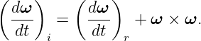
For the angular velocity vector itself,
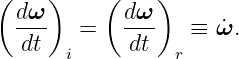
But
so the inertial and rotating derivatives of this angular velocity vector are equal:
Also,
Therefore
Expanding the last cross product,
8.3 Collecting the terms
Substitution gives
Thus
This is the fundamental acceleration relationship for two frames that share an origin.
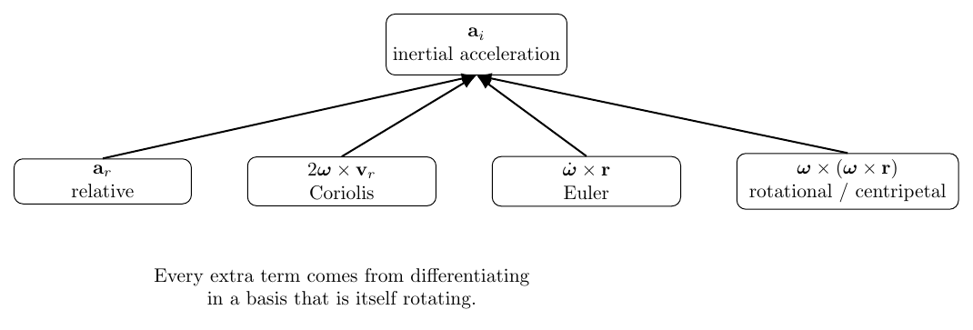
Figure. The acceleration decomposition for a point observed from a rotating frame.
Relative acceleration is supplemented by Coriolis, Euler, and rotational terms because the
observer’s basis is itself moving.
9 Interpreting each acceleration term
The equation
contains four physically different contributions.
9.1 Relative acceleration
is the acceleration measured relative to the rotating coordinates themselves.
9.2 Coriolis kinematic term
appears only when the object moves relative to the rotating frame. The factor of two arose because
one ω × vr term came from differentiating the relative velocity and another came from
differentiating the rotational transport velocity.
That factor of two is therefore not mysterious; it has a precise product-rule origin.
9.3 Euler term
appears when the rotating frame’s angular velocity itself changes. In mechanics this is
commonly called the Euler acceleration. It is unrelated to Euler Angles despite the shared
name.
9.4 Rotational centripetal term
is present even for a point fixed in the rotating frame.
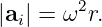
For rotation about the z axis and a position perpendicular to that axis,
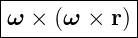
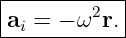
Use the vector triple-product identity:
Hence
It points inward. In the inertial acceleration decomposition it is therefore a centripetal
contribution.
10 Why centrifugal acceleration seems to have the opposite sign
The sign becomes different when Newton’s second law is written as an equation for the acceleration
observed in the rotating frame.
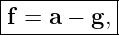
Suppose the frames share an origin and the inertial frame obeys
Substitute the rotating-frame decomposition:
Solve for mar:
The terms moved to the right-hand side are often described as inertial or apparent
forces.
Thus the rotating-frame apparent accelerations are
and
Since the double-cross term points inward, its negative points outward. This outward term is the
familiar centrifugal acceleration.
Therefore:
Keeping track of which equation is being written eliminates much of the usual sign
confusion.
11 Generalization to a translating and rotating origin
So far the two frames have shared an origin. A more general moving frame has an origin O that
translates relative to inertial frame i.
Let
be the inertial position of the moving origin, and let
be the position of point P measured from O in the rotating frame. Then
Differentiate once:
Differentiate again:
The new term
accounts for translational acceleration of the rotating frame’s origin.
This general form is important conceptually for local navigation frames. A local NED
frame not only rotates; its origin moves with the vehicle over the curved Earth. Later
lessons will organize those effects into Earth rate, transport rate, gravity, and position
kinematics.
12 Turntable example: where Coriolis curvature comes from
Consider a horizontal turntable rotating at constant angular velocity
A puck moves radially outward relative to the turntable with
The Coriolis contribution in the inertial acceleration decomposition is
Therefore
In the rotating-frame Newton equation the corresponding apparent acceleration is
Thus an observer on the turntable sees the freely moving puck deflect sideways even when no real
sideways force acts on it.
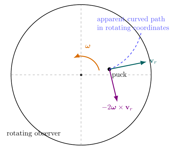
Figure. A puck moving across a rotating turntable. In inertial space its motion follows
ordinary Newtonian dynamics; in rotating coordinates the same trajectory appears curved,
and the rotating-frame equation contains the Coriolis term.
12.1 Numerical scale
Let
Then the Coriolis acceleration magnitude is
At radius
the centrifugal acceleration magnitude is
These are large because the turntable rate is deliberately high. Earth’s rotation is much slower, but
inertial navigation integrates small accelerations for long periods, so even modest rotating-frame
terms matter.
13 A point fixed to a uniformly rotating frame
A second diagnostic case is even simpler. Suppose
The inertial velocity is
and the inertial acceleration is
For r ⊥ ω,
The point therefore undergoes ordinary centripetal acceleration even though every coordinate of
the point is constant in the rotating frame.
This example is a useful reminder:
14 Connection with direction cosine matrices
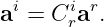
INS01 defined the passive DCM Cri that maps rotating-frame coordinates into inertial
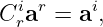
coordinates:
The columns of Cri are the rotating basis vectors expressed in inertial coordinates. Since each basis
vector obeys
the entire DCM satisfies
Differentiate
Using the DCM derivative then gives
Since
this is the coordinate-matrix form of the same transport theorem.
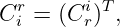
For the inverse DCM,
so
These identities are the direct bridge from rotating-frame mechanics to strapdown attitude
propagation. INS07 will extend them to the case in which both the body frame and navigation
frame rotate relative to inertial space.
15 Where this enters inertial navigation
The transport theorem appears repeatedly in the navigation problem.
15.1 Body frame
The IMU is physically attached to frame b. Its axes rotate with the vehicle. Gyroscope
measurements describe that rotation, and attitude propagation determines how body-resolved
measurements are transformed into a navigation frame.
15.2 Earth-fixed frame
Frame e rotates relative to inertial frame i with Earth angular rate
Consequently, derivatives in ECEF coordinates are not inertial derivatives.
15.3 Local navigation frame
The local-level frame n rotates both because Earth rotates and because the vehicle
moves across the curved Earth. Its total inertial angular rate is eventually decomposed
as
where
- ωien is Earth rotation resolved in n;
- ωenn is navigation-frame transport rate relative to Earth.
INS06 and INS13 will derive these quantities in detail.
15.4 Velocity equation
Repeated use of the transport theorem ultimately produces the rotating-frame terms in the
local-level strapdown velocity equation introduced in INS00:
INS02 does not yet derive this complete navigation equation. Its purpose is more fundamental:
every rotating-frame term in that equation should now have a mechanical origin rather than
appearing as unexplained notation.
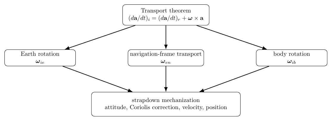
Figure. The transport theorem is the common geometric source of the rotating-frame
corrections that later appear in attitude and velocity mechanization.
16 Common sign and notation traps
16.1 Confusing ωir with ωri
By definition,
The transport theorem written here uses the angular velocity of the rotating frame r relative to
inertial frame i:
Reversing the angular-rate subscripts reverses the sign.
16.2 Calling the double-cross term centrifugal in every equation
In
the double-cross term points inward for a perpendicular radius and is the physical centripetal
contribution.
The outward centrifugal term appears only after this contribution is moved to the rotating-frame
side of Newton’s law.
16.3 Forgetting the factor of two in Coriolis acceleration
The factor of two comes from two different derivatives. One term arises when vr is differentiated in
a rotating basis and the second when ω × r is differentiated.
16.4 Forgetting translational acceleration of the moving origin
The simple four-term relation assumes a common origin. If the rotating frame origin translates,
add AOi explicitly.
16.5 Mixing coordinate derivatives with physical-vector derivatives
The expression
means the derivative of the r-resolved coordinate column. It is not generally the inertial derivative
of the physical vector.
17 Implementation checks suggested by the physics
Even before writing a complete inertial navigator, several tests should be used to validate
rotating-frame code.
17.1 Inertially fixed vector test
Choose a constant inertial vector and rotate the coordinate frame at known ω. The numerical
rotating-frame coordinates should satisfy
17.2 Rigidly rotating radius test
For a point fixed at radius r in a frame rotating at constant rate ω, verify
and
The acceleration must point toward the rotation axis.
17.3 Radial-motion Coriolis test
Give a point known radial velocity u in a frame rotating at ω and verify that the Coriolis
magnitude is
17.4 DCM derivative test
For a frame rotating at constant known angular velocity, verify numerically that
approaches zero at the expected integration order.
These tests will later become useful unit tests for strapdown mechanization software.
18 Where INS03 begins
INS02 has explained how derivatives change in rotating coordinates, but it has not yet answered a
different and equally important question:
A stationary accelerometer on a table reports approximately one g, while an accelerometer in
ballistic free fall reports approximately zero. This seems paradoxical if one assumes an
accelerometer directly measures kinematic acceleration.
INS03 will resolve that issue using proof-mass mechanics and Newton’s second law. The result will
be the specific-force relationship
which provides the translational input used by a strapdown inertial navigator.
19 Summary
For any physical vector a observed from inertial frame i and rotating frame r,
The result follows because every rotating basis vector satisfies
Applying the theorem to position gives
Applying it a second time gives
For a translating rotating origin O,
The same basis kinematics also gives the DCM derivative
These relationships are the Newtonian rotating-frame foundation on which Earth-fixed and
local-level strapdown navigation is built.
References
[1] David H. Titterton and John L. Weston, Strapdown Inertial Navigation Technology,
2nd ed., Institution of Electrical Engineers, 2004.
[2] Paul D. Groves, Principles of GNSS, Inertial, and Multisensor Integrated Navigation
Systems, 2nd ed., Artech House, 2013.
[3] Christopher Jekeli, Inertial Navigation Systems with Geodetic Applications, Walter
de Gruyter, 2001.
[4] Herbert Goldstein, Charles Poole, and John Safko, Classical Mechanics, 3rd ed.,
Addison-Wesley, 2002.
[5] Donald T. Greenwood, Principles of Dynamics, 2nd ed., Prentice-Hall, 1988.











![[ω] a = ω × a.
×](https://images.physicslibrary.org/cache/objects/1346/make4ht/StrapdownInertialNavigationTimeDerivativesInRotatingFrames21x.png)
![|---------------------------|
[( ) ]r |
| da- = a˙r + [ωrir]×ar. |
----dt--i--------------------](https://images.physicslibrary.org/cache/objects/1346/make4ht/StrapdownInertialNavigationTimeDerivativesInRotatingFrames22x.png)



















![F = m [ar + 2ω × vr + ω˙× r + ω × (ω × r )].](https://images.physicslibrary.org/cache/objects/1346/make4ht/StrapdownInertialNavigationTimeDerivativesInRotatingFrames57x.png)























![----------------
|˙i i i |
C-r-=-[ωir]×C-r.-](https://images.physicslibrary.org/cache/objects/1346/make4ht/StrapdownInertialNavigationTimeDerivativesInRotatingFrames85x.png)

![˙ai = [ωiir]×Cirar + Cira˙r.](https://images.physicslibrary.org/cache/objects/1346/make4ht/StrapdownInertialNavigationTimeDerivativesInRotatingFrames88x.png)
![|----------------|
|˙r r r |
C-i-=-−-[ω-ir]×C-i.-](https://images.physicslibrary.org/cache/objects/1346/make4ht/StrapdownInertialNavigationTimeDerivativesInRotatingFrames91x.png)






![˙ar = − [ωr ] ar.
ir×](https://images.physicslibrary.org/cache/objects/1346/make4ht/StrapdownInertialNavigationTimeDerivativesInRotatingFrames99x.png)


![˙i i i
Cr − [ωir]×Cr](https://images.physicslibrary.org/cache/objects/1346/make4ht/StrapdownInertialNavigationTimeDerivativesInRotatingFrames103x.png)




![|-i-----i----i-|
C˙r-=-[ωir]×C-r.-](https://images.physicslibrary.org/cache/objects/1346/make4ht/StrapdownInertialNavigationTimeDerivativesInRotatingFrames111x.png)