Strapdown Inertial Navigation: Vectors, Coordinate Frames, and Direction Cosine Matrices
A strapdown inertial navigator spends much of its life transforming the components of physical
vectors from one coordinate frame to another. Gyroscopes and accelerometers report
measurements in the body frame, while gravity models, Earth rotation, velocity, and
position are most naturally expressed in Earth-fixed or local navigation frames. Before any
time integration can be trusted, the coordinate transformations themselves must be
unambiguous.
This article develops the direction cosine matrix from first principles. The central distinction is
simple but fundamental:
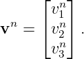
The geometric vector is independent of coordinates. A coordinate column is the set of
scalar projections of that vector onto a particular basis. Changing frames therefore
changes the numbers used to describe the vector without changing the vector itself. In this
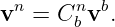
series that change of coordinates is represented by a passive direction cosine matrix
(DCM).
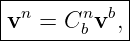
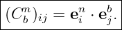
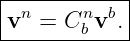
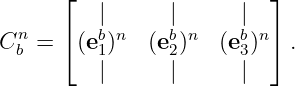
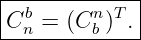
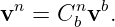
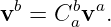
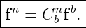
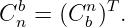
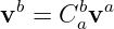
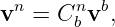
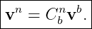
For the body and navigation frames,
where the subscript identifies the frame in which the coordinates begin and the superscript
identifies the frame in which they end. The same convention will be used for specific force,
gravity, Earth rate, transport rate, and every other vector quantity in the navigation
equations.
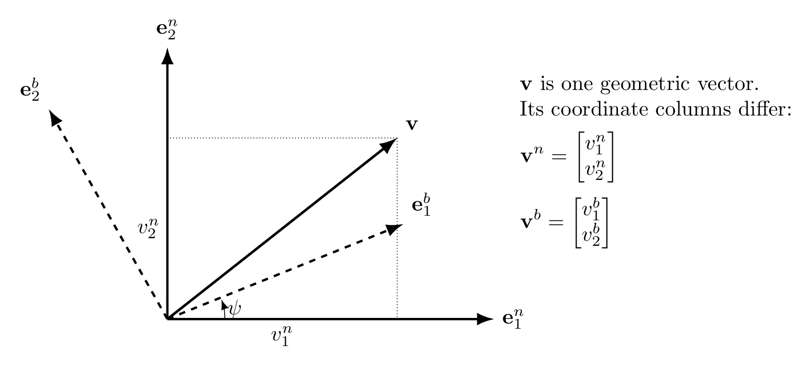
Figure. One geometric vector v can have different coordinate columns in two rotated
orthonormal frames. The vector itself has not moved; only the basis used to report its
components has changed.
The treatment follows the coordinate and attitude conventions commonly used in inertial-navigation
texts such as Titterton and Weston [1], Groves [2], and Jekeli [3]. Rotation-matrix and
attitude-representation issues are also discussed in the broader attitude literature, for example
Shuster [4] and Markley and Crassidis [5].
1 Learning objectives
After completing this entry, the reader should be able to:
- distinguish a geometric vector from its coordinate representation;
- define a coordinate frame as an ordered orthonormal basis;
- recover vector components by projection onto basis vectors;
- derive the passive DCM Cbn directly from basis-vector dot products;
- interpret each DCM entry as a direction cosine;
- prove that a DCM is orthogonal and that (Cbn)−1 = (C
bn)T = C
nb;
- explain why a proper DCM has determinant +1;
- compose coordinate transformations correctly and explain why matrix order matters;
- distinguish passive coordinate transformation from active rotation of a physical vector;
- define the skew-symmetric cross-product matrix [a]×;
- prove the identity
- transform a body-frame velocity or specific-force vector into NED coordinates;
- identify numerical invariants that can be used to test an implemented attitude
matrix.
2 The geometric vector comes first
Consider a velocity vector v. Its geometric meaning is independent of any coordinate system: it has
a magnitude and a direction in physical space. To perform numerical calculations, however, we
select an ordered basis
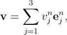
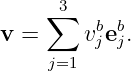
and write
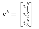
The coordinate column is
The superscript b does not create a new physical vector. It records which basis was used to obtain
the three scalar components.
If the same physical vector is resolved in the navigation basis
then
with a generally different coordinate column
The fundamental coordinate problem is therefore:
3 A coordinate frame is an ordered orthonormal basis
For the attitude transformations used in conventional strapdown navigation, the coordinate axes
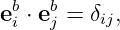
are mutually perpendicular unit vectors. Thus
and similarly
where δij is the Kronecker delta.
The order of the basis vectors matters. For the body frame we will commonly use
while the local navigation frame is
Both are right-handed frames. In particular,
This handedness condition will later distinguish a physical rotation matrix, whose determinant is
+1, from a general orthogonal matrix that could also represent a reflection.
4 Components are obtained by projection
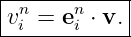
Because the basis is orthonormal, the coefficient multiplying a basis vector is obtained by taking a
dot product with that basis vector. Starting from
take the dot product with ein:
| ein ⋅ v | = e
in ⋅∑
j=13v
jne
jn | (16)
|
| = ∑
j=13v
jn | (17)
|
| = ∑
j=13v
jnδ
ij | (18)
|
| = vin. | (19) |
Therefore
This projection formula is the entire geometric foundation of the DCM.
5 Deriving the direction cosine matrix
Write the physical vector in body coordinates:
The ith navigation-frame component is
| vin | = e
in ⋅ v | (22)
|
| = ein ⋅∑
j=13v
jbe
jb | (23)
|
| = ∑
j=13 vjb. vjb. | (24) |
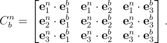
Define
Then the three component equations combine into
Thus
For unit vectors,
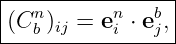
where 𝜃ij is the angle between the corresponding axes. This is why the matrix is called a direction
cosine matrix.
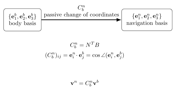
Figure. Every DCM element is a projection of one frame axis onto another. The entire
coordinate transformation follows directly from those nine dot products.
6 Matrix form using basis matrices
A compact derivation is useful because it makes several later proofs immediate. Represent both
orthonormal bases in any common orthonormal ambient basis and place their basis vectors into
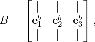
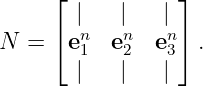
column matrices:
and
Because both bases are orthonormal,
If v denotes the physical vector expressed in the common ambient coordinates, then
and
Therefore
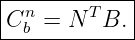
Comparing with the definition of the DCM gives
This expression makes the row-column interpretation transparent:
- column j of Cbn is the jth body axis expressed in navigation coordinates;
- row i of Cbn contains the projections of all body axes onto the ith navigation axis.
In particular,
That column interpretation is extremely useful when building a DCM from known reference
directions.
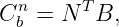
7 Orthogonality of a DCM
A proper attitude transformation preserves lengths and angles. We can prove this algebraically
from the basis construction.
Using
its transpose is
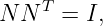
Then
| (Cbn)T C
bn | = BT NNT B. | (39) |
Since N is an orthogonal basis matrix,
so
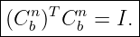
| (Cbn)T C
bn | = BT B | (41)
|
| = I. | (42) |
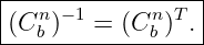
Thus
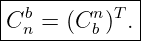
A square matrix satisfying this relationship is orthogonal. Therefore
The reverse coordinate transformation is consequently
This is one of the most useful identities in strapdown software. A separate general matrix inversion
should never be required to reverse a valid DCM transformation.
8 A DCM preserves vector length
Let
Then
| ∥vn∥2 | = (vn)T vn | (47)
|
| = (vb)T (C
bn)T C
bnvb | (48)
|
| = (vb)T vb | (49)
|
| = ∥vb∥2. | (50) |
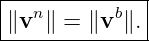
Hence
This is exactly what we expect: changing coordinates cannot change the physical speed,
acceleration magnitude, gravity magnitude, or angular-rate magnitude.
The same proof shows that dot products are preserved. If
then
| (an)T cn | = (ab)T (C
bn)T C
bncb | (53)
|
| = (ab)T cb. | (54) |
Thus angles between vectors are also unchanged by a passive coordinate transformation.
9 Why the determinant is +1
Orthogonality alone implies
so
A determinant of −1 corresponds to an improper orthogonal transformation such as a reflection. A
physical attitude transformation between two right-handed Cartesian frames is a proper rotation
and therefore satisfies
The set of all such matrices is the special orthogonal group
The notation SO(3) becomes increasingly useful when discussing finite rotations, quaternions,
rotation vectors, and numerical attitude propagation.
10 Composing coordinate transformations
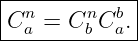
Suppose a vector is known in frame a and we want its components in frame n, but an intermediate
frame b is convenient. First transform from a to b:
Then transform from b to n:
Substitution gives
Therefore
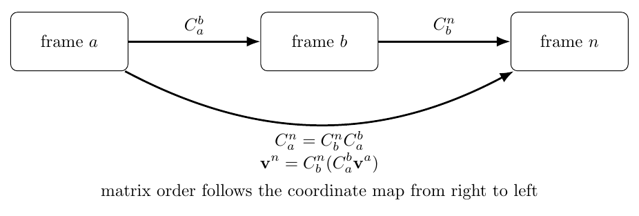
Figure. Coordinate transformations compose in the same order in which the coordinate
maps are applied, but matrix multiplication acts from right to left on the coordinate
column.
This rule is an important defense against frame-order errors. The adjacent frame labels cancel
visually:
The notation behaves somewhat like dimensional analysis: if the neighboring frame labels do not
match, the multiplication is probably not the transformation intended.
11 A two-dimensional derivation fixes the sign convention
Before using a three-dimensional attitude matrix, it is useful to derive a planar example.
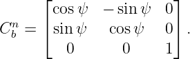
Let frame b be obtained from frame n by a positive right-handed rotation ψ about the
common positive third axis. Then the body axes expressed in navigation coordinates
are
and
Placing those vectors into the columns of the DCM gives
Its transpose is
Notice that both matrices are familiar “rotation matrices.” The notation tells us which coordinate
map is actually being performed.
12 Passive transformation versus active rotation
The same numerical matrix can appear in two conceptually different operations.
In a passive transformation, the physical vector is fixed and the basis changes:
In an active rotation, the basis is fixed and the physical vector itself is rotated:
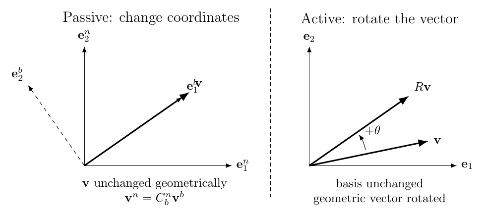
Figure. Passive and active rotations can use matrices with identical numerical entries
while representing different geometric operations. In strapdown mechanization, frame
superscripts and subscripts are used to keep the passive coordinate interpretation explicit.
This distinction is a frequent source of sign and transpose errors. Statements such as “rotate by
30∘” are incomplete unless they specify whether a vector is being actively rotated or whether
coordinates are being passively transformed into another frame.
For the convention used throughout this INS series,
13 A NED heading example
Consider a level vehicle whose body x axis points 30∘ east of north. With body axes
forward-right-down and navigation axes north-east-down,
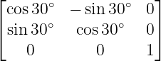
The body axes expressed in NED coordinates give
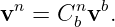
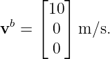
Suppose the vehicle velocity is purely forward in body coordinates:
Then
| vn | = C
bnvb | (74)
|
| =   | (75)
|
| =  m∕s. m∕s. | (76) |
Thus the vehicle has approximately 8.66 m/s north velocity and 5.00 m/s east velocity.
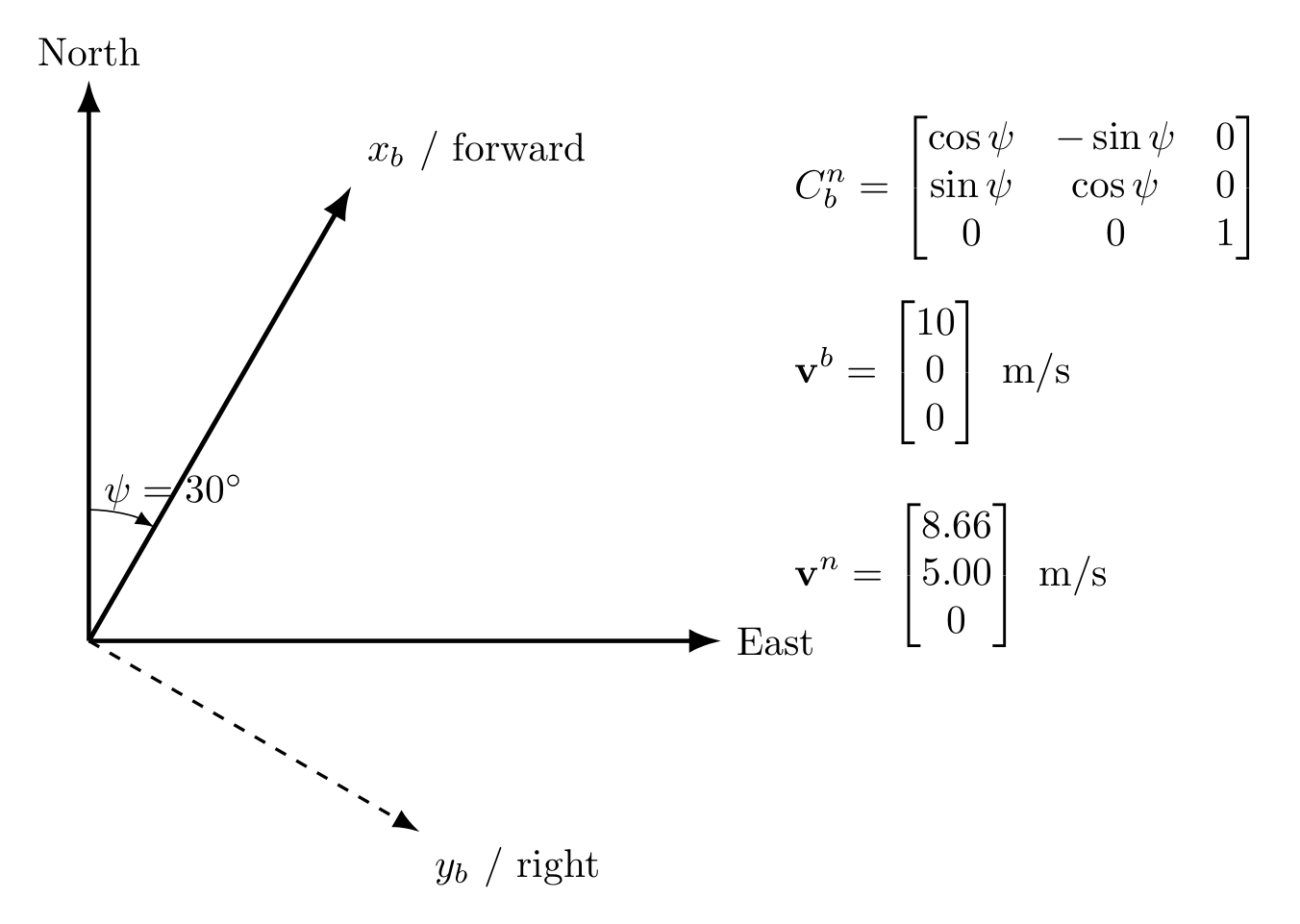
Figure. A level vehicle heading 30∘ east of north. A purely forward body-frame vector
becomes a combination of north and east components after multiplication by Cbn.
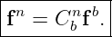
The same transformation is exactly what the strapdown navigator will apply to accelerometer
specific force:
Attitude is therefore the bridge between rotational sensing and translational navigation.
14 Cross products in matrix form
Rotating-frame mechanics contains many cross products. It is convenient to represent the
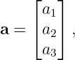
cross-product operation by a skew-symmetric matrix. For
define
Then for any vector b,
The matrix is skew-symmetric:
This notation lets rotational kinematics be written compactly and will appear throughout INS02
and the attitude-propagation articles.
15 A DCM preserves cross products
A proper rotation preserves both metric geometry and handedness. Therefore
Using skew-matrix notation,
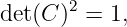
Since this is true for every cb,
Multiply on the right by
to obtain the identity
This is not merely a matrix trick. It says that “take the cross product with a” is itself a geometric
operation whose matrix representation must transform consistently when the coordinate basis
changes.
16 Small rotations and the first-order DCM
Although full attitude propagation is postponed to later articles, one first-order result
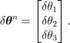
is useful now. Suppose frame b differs from frame n by a small right-handed rotation
vector
To first order, the body axes are obtained by rotating the navigation axes through the small
vector. The corresponding passive transformation from body coordinates to navigation coordinates
is
The inverse map is therefore
Terms quadratic in the small angles have been neglected. This approximation will become central
when deriving attitude-error dynamics and when connecting gyro bias to navigation
error.
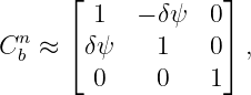
As a quick check, take a small positive yaw δψ about Down:
Then
which is exactly the first-order expansion of the planar DCM derived earlier.
17 Why a DCM contains nine numbers but only three degrees of freedom
A general 3 × 3 matrix contains nine independent scalar entries. A DCM cannot vary freely
because it must satisfy
The three columns must each have unit length, providing three constraints, and each pair of
distinct columns must be orthogonal, providing three additional constraints. Thus six independent
constraints reduce the nine entries to
independent rotational degrees of freedom.
This is why attitude can also be parameterized using three Euler Angles locally. Quaternions use
four scalars but impose one unit-norm constraint, again leaving three physical degrees of freedom.
Different attitude representations package the same three-dimensional rotational geometry in
different numerical forms [4, 5].
The DCM is particularly useful for derivation because the action on vectors is direct and frame
meaning remains visible. Quaternions will become especially useful for numerical propagation
because they avoid some singularities and preserve attitude efficiently with only four stored
numbers.
18 The DCM inside the strapdown mechanization
INS00 introduced the translational chain
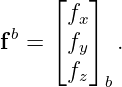
We can now interpret the first transformation exactly. The accelerometers measure the components
of the specific-force vector along the body axes:
The vector itself exists physically independent of coordinates. Multiplication by the attitude
DCM produces the components of the same specific-force vector along North, East, and
Down:
No force has been created by this multiplication. No physical vector has been rotated. The
navigation computer has simply re-expressed the accelerometer-measured vector in the coordinate
basis required by the velocity equation.
The same logic applies to angular velocity. If Earth rate is available in Earth-frame coordinates
and must be used in navigation coordinates, an appropriate DCM changes only the component
representation. Much of strapdown navigation can be understood as disciplined bookkeeping of this
type, coupled to physical differential equations.
19 Useful implementation checks
Because a DCM has strong geometric structure, several inexpensive tests can catch implementation
errors.
19.1 Orthogonality check
Compute
For a valid numerically propagated DCM, the entries of EC should remain close to zero. A
convenient scalar diagnostic is the Frobenius norm
Growth in this quantity indicates loss of orthogonality through numerical integration or coding
error.
19.2 Determinant check
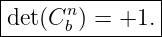
A proper attitude matrix should satisfy
A value near −1 indicates an axis reflection or handedness error, not a valid attitude.
19.3 Norm-preservation check
For a test vector,
A large difference indicates that the transformation is not orthogonal.
19.4 Round-trip check
Transform a vector from b to n and back:
The result should satisfy
This is an especially useful unit test because it simultaneously checks frame ordering and transpose
logic.
20 Common mistakes
20.1 Treating the coordinate column as the physical vector
The numbers in vb and vn differ even though the geometric vector is the same. Statements such as
“the vector changed after multiplication by the DCM” should therefore be avoided when discussing
a passive transformation.
20.2 Reading the frame labels backward
In this series,
means
Remembering this rule is more reliable than memorizing signs in particular matrices.
20.3 Using a transpose without stating why
The transpose reverses a DCM because the matrix is orthogonal:
This is a geometric property, not an arbitrary convention.
20.4 Multiplying transformations in the wrong order
If
and
then
not the reverse product.
20.5 Mixing active and passive descriptions
A matrix that actively rotates a vector by +𝜃 can have the same numerical entries as a passive
change of coordinates between frames separated by +𝜃. The physical interpretation must be
carried by explicit frame notation.
20.6 Ignoring handedness
An orthogonal matrix with determinant −1 preserves lengths but includes a reflection. It is not a
proper attitude DCM between two right-handed frames.
21 Where INS02 begins
Everything in this article concerns coordinate geometry at an instant of time. The frames may
have different orientations, but we have not yet asked how a vector derivative changes when the
basis itself rotates.
That is the central question of INS02.
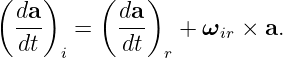
If a vector a is observed from an inertial frame and from a rotating frame, the derivatives are
related by the transport theorem
INS02 will derive this result directly from the time derivatives of rotating basis vectors and then
apply it twice to position. Coriolis, centrifugal, and Euler acceleration will emerge from that
derivation rather than being introduced as memorized correction terms.
The DCM and skew-matrix identities developed here provide the algebraic language required for
that derivation.
22 Summary
A physical vector exists independently of coordinates. In an orthonormal frame, its coordinate
components are obtained by projection onto the basis vectors:
The passive direction cosine matrix from frame b to frame n is therefore
and transforms coordinates according to
A DCM is a proper orthogonal matrix:
so
Coordinate transformations compose as
For rotational dynamics, the cross-product matrix
obeys
These results establish the coordinate language needed to derive rotating-frame kinematics in
INS02 and, ultimately, the full strapdown attitude and velocity equations.
References
[1] David H. Titterton and John L. Weston, Strapdown Inertial Navigation Technology,
2nd ed., Institution of Electrical Engineers, 2004.
[2] Paul D. Groves, Principles of GNSS, Inertial, and Multisensor Integrated Navigation
Systems, 2nd ed., Artech House, 2013.
[3] Christopher Jekeli, Inertial Navigation Systems with Geodetic Applications, Walter
de Gruyter, 2001.
[4] Malcolm D. Shuster, “A Survey of Attitude Representations,” The Journal of the
Astronautical Sciences, Vol. 41, No. 4, pp. 439–517, 1993.
[5] F. Landis Markley and John L. Crassidis, Fundamentals of Spacecraft Attitude
Determination and Control, Springer, 2014.


![n b n b b
[Cb a ]× = C b [a ]×C n;](https://images.physicslibrary.org/cache/objects/1344/make4ht/StrapdownInertialNavigationVectorsCoordinateFramesAndDirectionCosineMatrices2x.png)




















![[ ]
(eb1)n = cosψ ,
sin ψ](https://images.physicslibrary.org/cache/objects/1344/make4ht/StrapdownInertialNavigationVectorsCoordinateFramesAndDirectionCosineMatrices50x.png)
![[ ]
bn − sin ψ
(e 2) = cosψ .](https://images.physicslibrary.org/cache/objects/1344/make4ht/StrapdownInertialNavigationVectorsCoordinateFramesAndDirectionCosineMatrices51x.png)
![|-----[--------------]--|
| n cos ψ − sinψ |
C b = sinψ cosψ . |
-------------------------](https://images.physicslibrary.org/cache/objects/1344/make4ht/StrapdownInertialNavigationVectorsCoordinateFramesAndDirectionCosineMatrices52x.png)
![[ ]
Cbn = cosψ sin ψ .
− sinψ cosψ](https://images.physicslibrary.org/cache/objects/1344/make4ht/StrapdownInertialNavigationVectorsCoordinateFramesAndDirectionCosineMatrices53x.png)



![|------⌊----------------⌋--|
| 0 − a3 a2 |
[a] = ⌈ a 0 − a ⌉ .|
| × 3 1 |
---------−-a2--a1-----0-----](https://images.physicslibrary.org/cache/objects/1344/make4ht/StrapdownInertialNavigationVectorsCoordinateFramesAndDirectionCosineMatrices65x.png)
![|--------------|
[a]×b-=--a ×-b.-](https://images.physicslibrary.org/cache/objects/1344/make4ht/StrapdownInertialNavigationVectorsCoordinateFramesAndDirectionCosineMatrices66x.png)
![T
[a]× = − [a ]×.](https://images.physicslibrary.org/cache/objects/1344/make4ht/StrapdownInertialNavigationVectorsCoordinateFramesAndDirectionCosineMatrices67x.png)

![Cnb [ab]×cb = [Cnb ab]×Cnb cb.](https://images.physicslibrary.org/cache/objects/1344/make4ht/StrapdownInertialNavigationVectorsCoordinateFramesAndDirectionCosineMatrices69x.png)
![n b n b n
Cb [a ]× = [C b a ]×Cb .](https://images.physicslibrary.org/cache/objects/1344/make4ht/StrapdownInertialNavigationVectorsCoordinateFramesAndDirectionCosineMatrices70x.png)

![|----------------------|
-[Cnb ab]×-=-Cnb [ab]×Cbn.](https://images.physicslibrary.org/cache/objects/1344/make4ht/StrapdownInertialNavigationVectorsCoordinateFramesAndDirectionCosineMatrices72x.png)
![|----------------|
Cnb ≈ I + [δ𝜃n]×.|
------------------](https://images.physicslibrary.org/cache/objects/1344/make4ht/StrapdownInertialNavigationVectorsCoordinateFramesAndDirectionCosineMatrices74x.png)
![Cbn ≈ I − [δ𝜃n]×.](https://images.physicslibrary.org/cache/objects/1344/make4ht/StrapdownInertialNavigationVectorsCoordinateFramesAndDirectionCosineMatrices75x.png)
![⌊ ⌋
0 − δ ψ 0
[δ𝜃 ]× = ⌈δψ 0 0⌉ .
0 0 0](https://images.physicslibrary.org/cache/objects/1344/make4ht/StrapdownInertialNavigationVectorsCoordinateFramesAndDirectionCosineMatrices76x.png)














![[a ]×b = a × b](https://images.physicslibrary.org/cache/objects/1344/make4ht/StrapdownInertialNavigationVectorsCoordinateFramesAndDirectionCosineMatrices102x.png)
![|----------------------|
| n b n b b |
-[Cb a-]×-=-C-b [a-]×C-n.](https://images.physicslibrary.org/cache/objects/1344/make4ht/StrapdownInertialNavigationVectorsCoordinateFramesAndDirectionCosineMatrices103x.png)