1 Where GPSORB02 fits in the derivation chain
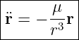
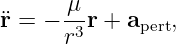
GPSORB01 derived the ideal Earth-satellite relative equation
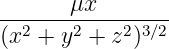
from Newton’s second law and universal gravitation. Written in Cartesian coordinates,
Kaplan’s discussion then leads toward six orbital elements. The natural question is:
Why does Eq. (1), which looks like one vector equation, require six independent
constants to determine one satellite trajectory?
The short answer is that Eq. (1) contains three coupled second-order scalar equations. Each
second-order degree of freedom contributes two initial data: position and velocity. The
purpose of this article is to make that counting rigorous and then connect it to orbital
geometry.
2 Begin in one dimension: why second order means two constants
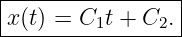
Consider the simplest second-order differential equation,
Integrating once gives
and integrating again gives
Two arbitrary constants appear because the equation is second order. If the position and velocity
are specified at t = t0,
then
Thus the two constants may be represented either as abstract integration constants (C1,C2) or as
physically meaningful initial data (x0,v0).
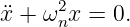
A harmonic oscillator makes the same point in a less trivial way:
Its general solution is
Again there are two constants. One may instead use amplitude and phase,
which shows an important principle for orbital mechanics:
The number of independent constants is fixed by the differential equation, but
the coordinates used to represent those constants are not unique.
The pair (A,B) and the pair (C,ϕ) describe the same two-dimensional family of solutions.
3 Three dimensions: the two-body problem has a six-dimensional state
Introduce the velocity
and define the state vector
Equation (1) is then equivalent to the first-order system
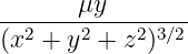
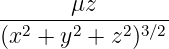
In components,
 | = vx, |  | = vy, |  | = vz, | (14)
|
 | = − , , |  | = − , , |  | = − . . | (15) |
A unique solution is selected by specifying all six state components at one epoch t0:
Thus the initial condition consists of
These are six independent scalar quantities.
For r≠0, the right-hand side of Eq. (13) is smooth, so the usual existence-and-uniqueness theorem
for ordinary differential equations guarantees a locally unique trajectory through a specified state.
Symbolically one may write the resulting flow as
The solution family therefore has six parameters because x0 belongs to a six-dimensional state
space.
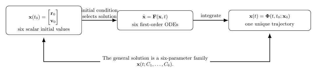
Figure 1. The two-body equation is a six-state first-order system. Six scalar initial values select
one trajectory from the six-parameter family of possible solutions.
4 What “six constants of integration” really means
For a general coupled nonlinear system such as Eq. (13), one should not imagine literally
integrating the x, y, and z equations twice independently. The components are coupled
through
The phrase “six constants of integration” is better understood structurally:
-
1.
- the system has six first-order state equations;
-
2.
- a general local solution therefore depends on six independent parameters;
-
3.
- specifying six independent initial values fixes those parameters;
-
4.
- any other nonsingular set of six coordinates may be used instead.
We may denote a general solution abstractly by
The constants Ci need not look like Cartesian coordinates. They may be transformed into
quantities with much more physical meaning.
This is precisely what orbital elements do.
5 Constants of integration are not the same as constants of motion
Two phrases sound similar but should be distinguished.
A constant of integration is an arbitrary parameter required to identify one member
of a family of differential-equation solutions. Initial position and initial velocity are
examples.
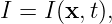
A constant of motion, also called a first integral or invariant, is a function of the state that remains
constant along a trajectory. If
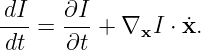
then along the motion
If
then I is constant along that solution.
The distinction matters because one can have several components of conserved vectors without all
of them being independent. Conversely, not every constant needed to specify the time history must
appear as a familiar conserved scalar.
6 The special constants of the Kepler problem
The inverse-square central-force problem has unusually rich structure. Later articles derive the
conservation laws in detail; here we introduce them to understand the counting.
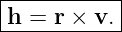
6.1 Specific angular momentum
Define
For the central two-body force, h is constant. Its direction is normal to the orbital plane, so two
directional degrees of freedom orient that plane, while its magnitude contains information about
the orbit’s transverse motion.
Although h has three Cartesian components,
it is one conserved vector, not three unrelated conservation laws.
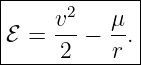
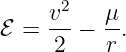
6.2 Specific mechanical energy
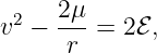
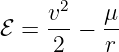
Define
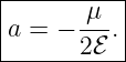
For the ideal two-body problem, ℰ is constant. For an ellipse it later gives the semimajor axis
through
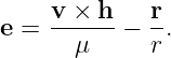
6.3 Eccentricity vector
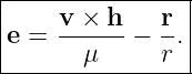
Define
For the inverse-square two-body problem, e is constant. Its magnitude
is the orbital eccentricity, and its direction points toward periapsis.
At first glance we now seem to have
constants. But the original differential equation only requires six parameters, and even those six
include orbital phase. Something is clearly being overcounted.
7 Why the conserved quantities are constrained
The conserved quantities in the Kepler problem are not all independent.
7.1 First constraint: h is perpendicular to e
Take the dot product of Eqs. (24) and (28):
| h ⋅ e | =  h ⋅ (v × h) − h ⋅ h ⋅ (v × h) − h ⋅ . . | (31) |
The first term vanishes because v × h is perpendicular to h. The second vanishes because
is perpendicular to r. Hence
Thus the six components of h and e satisfy at least one algebraic constraint.
7.2 Second relation: energy is determined by h and e
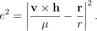
Square the eccentricity-vector definition:
Expanding,
Because v ⋅ h = 0,
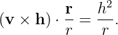
Next use the vector triple-product identity
Dotting with r gives
| (v × h) ⋅ r | = r2v2 − (r ⋅ v)2, | (38)
|
| = |r × v|2, | (39)
|
| = h2. | (40) |
Therefore
Substituting Eqs. (36) and (41) into Eq. (35),
| e2 | =  + 1 − + 1 − , , | (42)
|
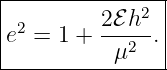
| = 1 +  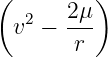 . . | (43) |
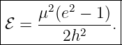
Using Eq. (26),
so
Equivalently,
Thus energy is not independent once the magnitudes of h and e are known.
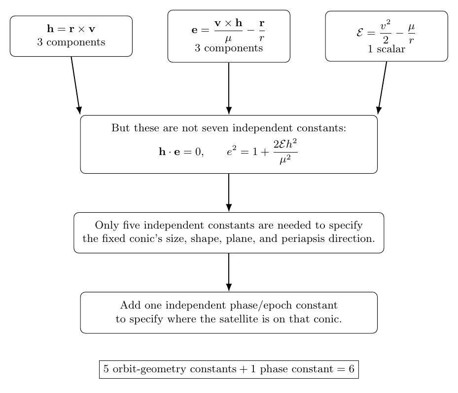
Figure 2. The conserved angular-momentum vector, eccentricity vector, and energy contain
redundant information. Their algebraic relations leave five independent constants describing the
fixed Keplerian conic. A sixth phase constant is still required for the complete time-dependent
solution.
8 Five constants determine the orbit curve, but not the satellite’s location
This is the central conceptual point of GPSORB02.
The fixed Keplerian conic in three-dimensional space requires five independent geometric
parameters:
-
1.
- one parameter for size;
-
2.
- one for shape;
-
3.
- two to orient the orbital plane;
-
4.
- one to orient periapsis within that plane.
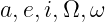
For an ellipse these are naturally represented by
But these five parameters specify only the curve. They do not tell us where the satellite is on the
curve at a particular time.
Imagine two satellites occupying different points on exactly the same ideal Keplerian ellipse with
the same direction of motion. They can have the same a,e,i, Ω, and ω. They also share the same h,
e, and specific orbital energy. Yet their position vectors at the same clock time are
different.
A sixth parameter is therefore required to specify orbital phase.
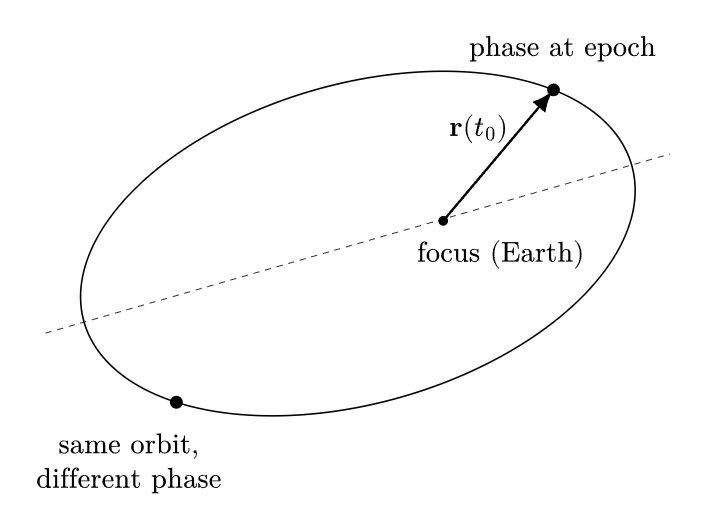
Figure 3. Five constants define the oriented Keplerian conic. One additional phase constant
specifies where the satellite is on that conic at a chosen epoch.
9 The sixth constant: phase or epoch information
Several equivalent quantities can supply the missing phase information. Common choices
include
or the time of periapsis passage
These are not four additional degrees of freedom. For a known Keplerian orbit they are alternative
representations of the same one-dimensional phase information.
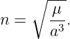
For an ellipse, later articles derive
and
where
Thus M0 is especially convenient because its ideal two-body propagation is linear in
time.
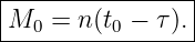
Another common representation is
so that
The constant M0 and the constant τ therefore encode the same phase degree of freedom once n
and t0 are fixed.
10 The six classical orbital elements
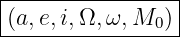
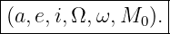
For a nondegenerate elliptical orbit, one standard six-element set is
Their roles can be organized as follows:
| Element | Role | Physical meaning |
| a | size | Semimajor axis; sets orbital energy and
characteristic period. |
| e | shape | Eccentricity; distinguishes circular and elliptical
shape within the bound case. |
| i | plane orientation | Inclination of the orbital plane relative to the
reference plane. |
| Ω | plane orientation | longitude or right ascension of
the ascending-node direction, depending on the
chosen reference frame. |
| ω | in-plane orientation | Argument of periapsis; rotates the ellipse within
its orbital plane. |
| M0 | phase | Mean anomaly at the chosen reference epoch t0;
locates the satellite in time along the orbit. |
The decomposition is therefore
This is the geometric meaning behind the six constants of the two-body solution.
11 Cartesian state and orbital elements are two coordinate systems for one state
At an epoch t0, the Cartesian description is
The classical-element description is
Away from classical-element singularities, there is a reversible transformation
The state has not acquired or lost information. We have merely changed coordinates in the
six-dimensional space of initial conditions.
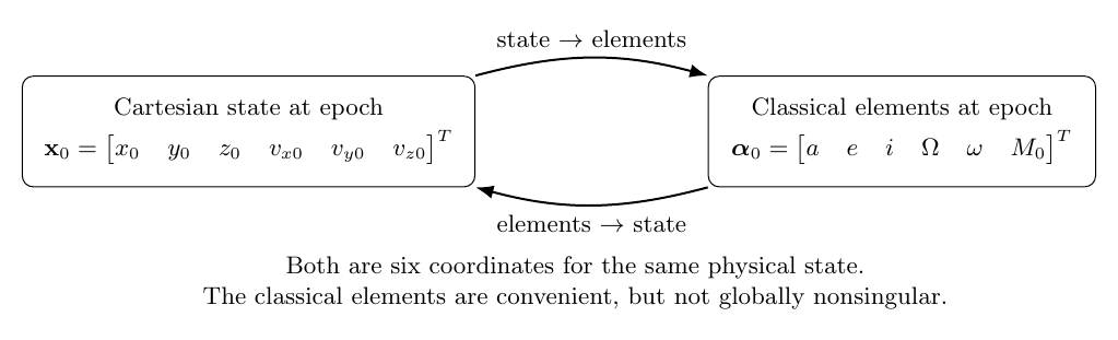
Figure 4. Cartesian state components and classical orbital elements are alternative six-parameter
descriptions of the same physical state, provided the orbital-element representation is nonsingular.
This viewpoint is valuable because it removes some of the mystery from orbital elements. They are
not six new physical laws. They are a coordinate transformation chosen because the resulting
numbers expose orbit geometry and make Keplerian propagation convenient.
12 How the state begins to reveal the elements
The complete state-to-element derivation is reserved for GPSORB05 and GPSORB07, but the
structure can already be previewed.
Given r and v, compute
The direction of h establishes the orbital plane and later yields i and Ω.
Compute
For an ellipse,
Compute the eccentricity vector
Then
and the direction of e identifies periapsis, allowing ω to be determined after the node direction is
known.
Finally, the angle or anomaly locating r relative to periapsis supplies the phase. Thus
the six Cartesian numbers are systematically reorganized into the six orbital-element
numbers.
13 Why the six elements are constant only in the ideal two-body problem
For Eq. (1), the classical Keplerian elements may be treated as constants except for the anomaly
that advances with time. More precisely, one may choose a constant phase-at-epoch such as M0
and use time to propagate the instantaneous anomaly.
For a real satellite, however,
where apert may contain nonspherical gravity, third-body gravity, solar radiation pressure,
maneuvers, and other effects. The orbital elements then become time-varying quantities,
One may interpret them as osculating elements: at each instant they describe the Keplerian conic
tangent to the real trajectory in state space.
This distinction is essential for GPS. The broadcast ephemeris uses parameters that are Keplerian
in appearance but are augmented by secular rates and periodic corrections so that a compact user
algorithm can reproduce the satellite’s fitted Earth-fixed trajectory over the intended
interval.
14 The bridge to the GPS broadcast ephemeris
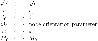
The six classical quantities explain the skeleton of the legacy GPS broadcast parameterization. In
the idealized limit, the following correspondences are suggestive:
The word “correspondence” is deliberate. The broadcast quantities should not be interpreted as six
untouched constants of an exact inertial Kepler ellipse. In the legacy LNAV user algorithm, for
example, Ω0 is defined relative to the GPS weekly epoch and is combined with Earth rotation and
the transmitted node rate. The broadcast values are fitting parameters for a specified user
model.
The additional legacy terms include
and the harmonic correction coefficients
These do not mean the underlying differential equation suddenly needs more than six initial
conditions. Instead, they belong to a compact parameterization of a perturbed and fitted trajectory
model. The fundamental dynamical state is still six-dimensional; the broadcast message uses
additional coefficients because it approximates time-varying departures from one fixed Keplerian
conic.
This distinction resolves an apparent paradox:
Six numbers are enough to specify an ideal two-body state, while more than six
transmitted coefficients may be useful to approximate a real GPS orbit over time.
15 A useful dimensional argument: orbit geometry versus orbital phase
There is another way to see the 5 + 1 structure without using any formulas.
An ellipse in its own plane requires two numbers to specify size and shape. Placing that
plane in three-dimensional space requires two orientation angles. Rotating the ellipse
within its plane requires one additional angle. This totals five numbers for the geometric
curve.
A moving satellite is not merely a curve. One must also specify a location along that curve at a
reference time. That is the sixth number.
This geometric counting exactly mirrors the differential-equation counting:
The agreement is not accidental. Both descriptions encode the same physical state.
16 Special cases and singular classical elements
The classical six-element set is intuitive but not globally well behaved.
16.1 Circular orbit
If
there is no unique periapsis direction. Consequently, ω is undefined. One instead uses
a combined angle such as argument of latitude or true longitude, depending on the
geometry.
16.2 Equatorial orbit
If
the orbital plane coincides with the reference equatorial plane. The line of nodes is not uniquely
defined, so Ω is undefined.
16.3 Circular equatorial orbit
If both
several classical angles lose separate meaning, although the Cartesian state itself remains perfectly
well defined.
This is an important mathematical point: the physical state space remains six-dimensional, but a
particular coordinate chart can become singular. Alternative element sets such as equinoctial
elements are designed to avoid some of these singularities.
GPS satellites normally have small but nonzero eccentricity and substantial inclination, so the
classical geometry remains very useful for understanding the broadcast equations. Still, one should
not confuse a coordinate singularity with a physical singularity.
17 A second caution: not every six-number list is independent
A set containing six numerical entries is not automatically a valid six-coordinate representation.
Independence matters.
For example, suppose one tried to use the six components
These six quantities satisfy
so they cannot vary independently. They describe only a five-dimensional family of Keplerian orbit
geometries. A separate phase quantity must still be supplied.
Similarly, adding energy to the list does not create a new independent degree of freedom because of
Eq. (45).
This is why careful orbit mechanics counts independent constants rather than merely counting
symbols.
18 Worked conceptual example: same orbit, different state
Consider two satellites A and B on the same ideal Keplerian ellipse. Suppose they have the
same
and move in the same direction. Then they share the same orbital plane, semimajor axis,
eccentricity, periapsis direction, specific energy, angular momentum vector, and eccentricity
vector.
Let their mean anomalies at epoch differ:
Then
in general. The five geometry constants are identical, but the six-dimensional states are
different.
This example shows precisely why the invariants that determine the conic are not enough to
specify a time-tagged satellite state.
19 What will be derived next
GPSORB02 has established the dimensional and mathematical structure without yet relying on
the detailed derivation of each conservation law. The next articles can now proceed in a clean
sequence.
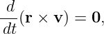
GPSORB03 will start from Eq. (1) and derive
so that
is constant. From this, the planarity of two-body motion and Kepler’s area law will
follow.
GPSORB04 will derive conservation of
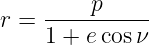
and the eccentricity vector, leading to the conic equation
and the relations
Those derivations will turn the abstract “six constants” discussed here into concrete orbital
geometry.
20 Summary
The ideal satellite equation
is three coupled second-order equations, equivalently six first-order equations. Therefore one unique
trajectory requires six independent scalar initial values,
These six numbers may be replaced by any nonsingular six-parameter coordinate system describing
the same state.
The Kepler problem supplies conserved angular momentum, eccentricity, and energy, but those
quantities are not all independent:
Five independent constants specify the fixed conic’s size, shape, and orientation. A sixth phase
constant specifies where the satellite is on the conic at an epoch. This produces the classical
structure
and explains why these six quantities are a natural bridge between Newton’s equation of motion
and the GPS broadcast ephemeris.
The key conceptual chain is
References
[1] E. D. Kaplan and C. J. Hegarty, editors, Understanding GPS: Principles and
Applications, 2nd ed., Artech House, 2006.
[2] R. R. Bate, D. D. Mueller, and J. E. White, Fundamentals of Astrodynamics, Dover
Publications, 1971.
[3] D. A. Vallado, Fundamentals of Astrodynamics and Applications, 4th ed., Microcosm
Press, 2013.
[4] R. H. Battin, An Introduction to the Mathematics and Methods of Astrodynamics,
revised ed., AIAA Education Series, 1999.
[5] H. D. Curtis, Orbital Mechanics for Engineering Students, 4th ed., Elsevier, 2020.
[6] O. Montenbruck and E. Gill, Satellite Orbits: Models, Methods, and Applications,
Springer, 2000.
[7] Global Positioning Systems Directorate, IS-GPS-200N: NAVSTAR GPS Space
Segment/Navigation User Interfaces, 1 August 2022.








![|----[-]---------------------------|
x = r = [x y z v v v ]T .
| v x y z |
------------------------------------](https://images.physicslibrary.org/cache/objects/1259/make4ht/SixConstantsOfOrbitalMotionFromInitialConditionsToOrbitalElements13x.png)
![|-----------[--------]--|
| v |
x˙= F(x) = − μr ∕r3 .|
-------------------------](https://images.physicslibrary.org/cache/objects/1259/make4ht/SixConstantsOfOrbitalMotionFromInitialConditionsToOrbitalElements14x.png)
![|------------[---]--|
| r0 |
x0 = x (t0) = v . |
----------------0----](https://images.physicslibrary.org/cache/objects/1259/make4ht/SixConstantsOfOrbitalMotionFromInitialConditionsToOrbitalElements24x.png)





![[ ]
h = hx hy hz T ,](https://images.physicslibrary.org/cache/objects/1259/make4ht/SixConstantsOfOrbitalMotionFromInitialConditionsToOrbitalElements33x.png)

















![[ ]
x0 = r0 ∈ ℝ6.
v0](https://images.physicslibrary.org/cache/objects/1259/make4ht/SixConstantsOfOrbitalMotionFromInitialConditionsToOrbitalElements67x.png)
![[ ]
α0 = a e i Ω ω M0 T .](https://images.physicslibrary.org/cache/objects/1259/make4ht/SixConstantsOfOrbitalMotionFromInitialConditionsToOrbitalElements68x.png)

















![[ ]
r0
x0 = v0 .](https://images.physicslibrary.org/cache/objects/1259/make4ht/SixConstantsOfOrbitalMotionFromInitialConditionsToOrbitalElements95x.png)