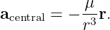
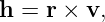
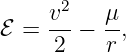
1 Where GPSORB01 fits in the derivation chain
GPSORB00 established the long path
The purpose of the present article is to make the first arrow rigorous.
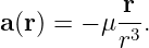
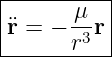
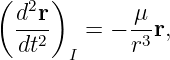
Kaplan and Hegarty write the ideal satellite equation of motion in the familiar form
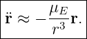
with r = ∥r∥. Equation (2) contains a remarkable amount of physics in one line. It assumes a
particular force law, a particular choice of coordinates, and an idealization of Earth and the
satellite. Before extracting orbital elements from it, we should understand exactly where every
factor comes from.
2 The physical two-body system
Consider an Earth of mass M and a satellite of mass m. We begin in a Newtonian inertial frame
with fixed, nonrotating axes. Let
| RM(t) | = position of Earth’s center of mass, | (3)
|
| Rm(t) | = position of the satellite’s center of mass. | (4) |
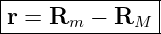
Define the relative position from Earth to satellite by
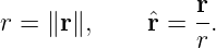
and its magnitude and unit vector by
Figure 1 shows the geometry.
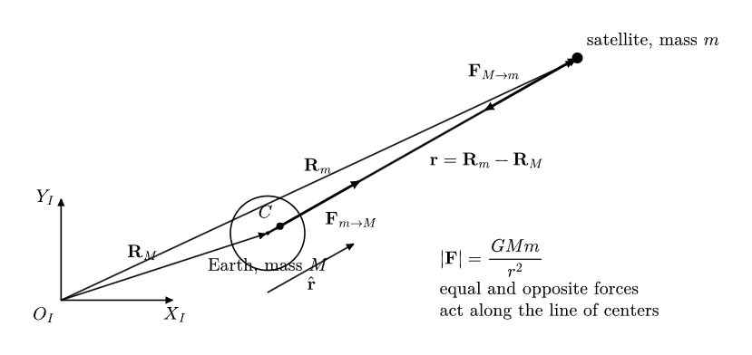
Figure 1. Exact Newtonian two-body geometry. The Earth and satellite both accelerate; the
relative vector is the quantity needed for orbital motion about Earth. Point C denotes the system
barycenter, which lies extremely close to Earth’s center for an artificial satellite.
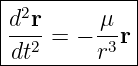
A key point is already visible: in the exact two-body problem, Earth is not perfectly fixed. The
satellite pulls on Earth with the same force magnitude that Earth exerts on the satellite. The
Earth-centered orbit equation will therefore emerge most cleanly from relative motion, not from
pretending at the outset that Earth cannot move.
3 Newton’s law of universal gravitation
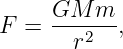
Newton’s universal gravitation law gives the magnitude of the attractive force between two point
masses separated by distance r:
where G is the universal gravitational constant.
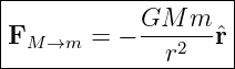
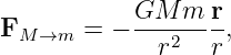
The force on the satellite points toward Earth, which is opposite the direction of r.
Therefore
Using Eq. (6),
so
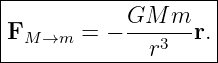
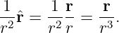
This is the source of the r3 in the vector equation. The magnitude still follows an inverse-square
law. Multiplying by the radial unit vector contributes one additional factor of 1∕r:
There is no inverse-cube force law hidden in Eq. (2).
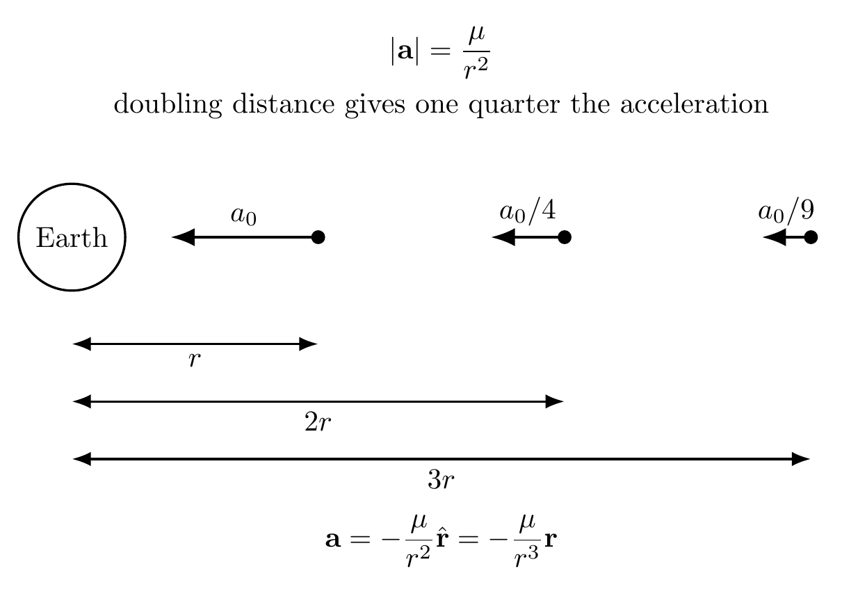
Figure 2 emphasizes the distinction between the vector expression and the physical inverse-square
magnitude.
4 Newton’s third law and the force on Earth
Newton’s third law gives an equal and opposite force on Earth:
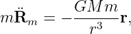
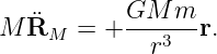
Applying Newton’s second law separately to both bodies gives
and
Canceling the corresponding masses yields
| Rm | = − r, r, | (15)
|
| RM | = + r. r. | (16) |
These are the accelerations of the two bodies with respect to the original inertial frame.
5 The exact relative-motion equation
Differentiate the definition of the relative vector, Eq. (5), twice:
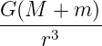
Substitute Eqs. (15) and (16):
| r | = − r − r − r, r, | (18)
|
| = − r. r. | (19) |
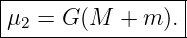
Define the exact two-body gravitational parameter
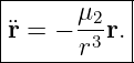
Then the exact relative-motion equation is
This result is worth pausing over. Equation (21) is not obtained by assuming Earth is
immovable. It follows from subtracting the two inertial equations of motion. The coordinate r
measures the separation between the bodies, and the parameter contains the sum of their
masses.
5.1 Why satellite texts usually write μ ≈ GM
For an artificial satellite,
Hence
and therefore
The relative equation becomes
This is the form used throughout basic satellite dynamics and is the physical origin of Kaplan’s
equation.
The approximation is extraordinarily good for a navigation satellite. Even a spacecraft mass of
several tonnes is negligible compared with Earth’s mass. The spacecraft’s own mass cancels from
the satellite acceleration equation and contributes negligibly to M + m in the exact relative
equation.
6 Center-of-mass motion: why the two-body problem separates
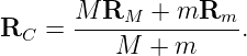
Define the system center of mass
Differentiate twice:
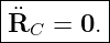
Using Eqs. (13) and (14), the internal gravitational forces cancel:
Therefore
The barycenter moves at constant velocity in an isolated two-body system.
The full motion therefore separates naturally into two pieces:
-
1.
- uniform translation of the center of mass; and
-
2.
- relative orbital motion governed by Eq. (21).
For orbital mechanics we normally discard the dynamically uninteresting uniform translation and
study the relative coordinate r.
7 Why a spherical Earth may be treated as a point mass
Newton’s inverse-square force law in Eqs. (8)–(10) was written as though all of Earth’s mass were
concentrated at one point. Why is this allowed for a satellite outside Earth?
Newton’s shell theorem states that a spherically symmetric mass distribution attracts an exterior
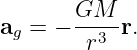
point mass exactly as if the entire mass were concentrated at the center. Thus for an ideal spherical
Earth, the external gravitational acceleration is
The real Earth is not perfectly spherical. It is oblate and has a nonuniform mass distribution.
Those departures generate the J2 and higher spherical-harmonic corrections introduced later in
GPSORB10. Equation (25) is therefore the central-body baseline model, not the final high-fidelity
GPS force model.
8 A second derivation from gravitational potential
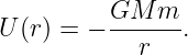
The same equation can be obtained from potential energy. For a satellite in the point-mass Earth
approximation, the gravitational potential energy is
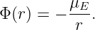
Divide by satellite mass to obtain the specific gravitational potential
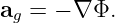
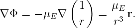
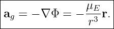
The gravitational acceleration is the negative gradient:
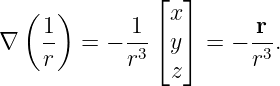
In Cartesian coordinates,
The derivative of 1∕r with respect to x is
  | =  (x2 + y2 + z2)−1∕2, (x2 + y2 + z2)−1∕2, | (35)
|
| = − (x2 + y2 + z2)−3∕2(2x), (x2 + y2 + z2)−3∕2(2x), | (36)
|
| = − . . | (37) |
Similarly,
Thus
Using Eq. (32),
Finally,
The force-law derivation and the potential-gradient derivation are mathematically equivalent. The
potential viewpoint becomes especially valuable when nonspherical gravity is added, because
additional gravitational structure is naturally represented by additional terms in the
potential.
9 Dimensional check
A useful engineering habit is to verify units before trusting a dynamical equation. The
gravitational parameter has dimensions
The factor r∕r3 has dimensions
Therefore
which is correctly an acceleration.
10 The role of the reference frame
Equation (25) is a Newtonian inertial-frame equation, or equivalently an equation for the
relative coordinate expressed in axes that are not rotating with Earth. This condition
matters.
Suppose a vector is represented in an inertial frame I and a frame E rotating with angular velocity
ΩE∕I. The transport theorem gives
Differentiate again:
 I = I = |  E + 2ΩE∕I × E + 2ΩE∕I × E E | (46)
|
| +  × r + ΩE∕I × × r + ΩE∕I ×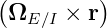 . . | (47) |
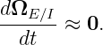
For nearly constant Earth rotation rate,
If the inertial acceleration is central gravity,
then the Earth-fixed coordinate acceleration satisfies
The additional terms are the Coriolis and centrifugal accelerations associated with the rotating
coordinates.
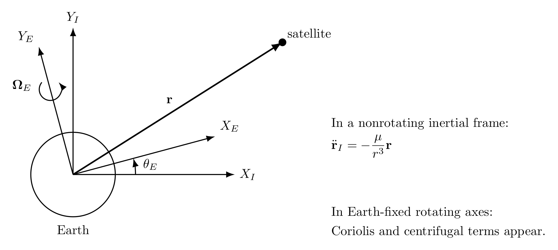
Figure 3. The central-force equation has its simplest form in nonrotating inertial axes. Expressing
motion in Earth-fixed rotating axes introduces additional kinematic terms.
This is why one must not casually label the components x,y,z as ECEF and still use Eq. (25)
unchanged. The force is the same physical gravity, but the coordinate acceleration is frame
dependent.
GPS broadcast ephemeris eventually produces Earth-fixed coordinates, so the inertial-to-rotating-frame
distinction will return in GPSORB09 and GPSORB15.
11 Cartesian component equations
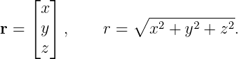
Let the nonrotating Cartesian coordinates of the relative vector be
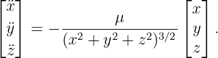
Then Eq. (25) becomes
Thus
| ẍ = −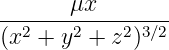 , , | (53)
|
| ÿ = −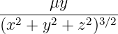 , , | (54)
|
| z = −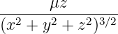 . . | (55) |
The equations are coupled and nonlinear. The x acceleration, for example, depends not only on x
but also on y and z through r.
12 From one second-order vector equation to six first-order equations
Numerical propagators and navigation filters usually work with first-order state equations. Define
velocity
and the six-component state
Then
In scalar form,
 | = vx, | (59)
|
 | = vy, | (60)
|
 | = vz, | (61)
|
 | = − , , | (62)
|
 | = − , , | (63)
|
 | = − . . | (64) |
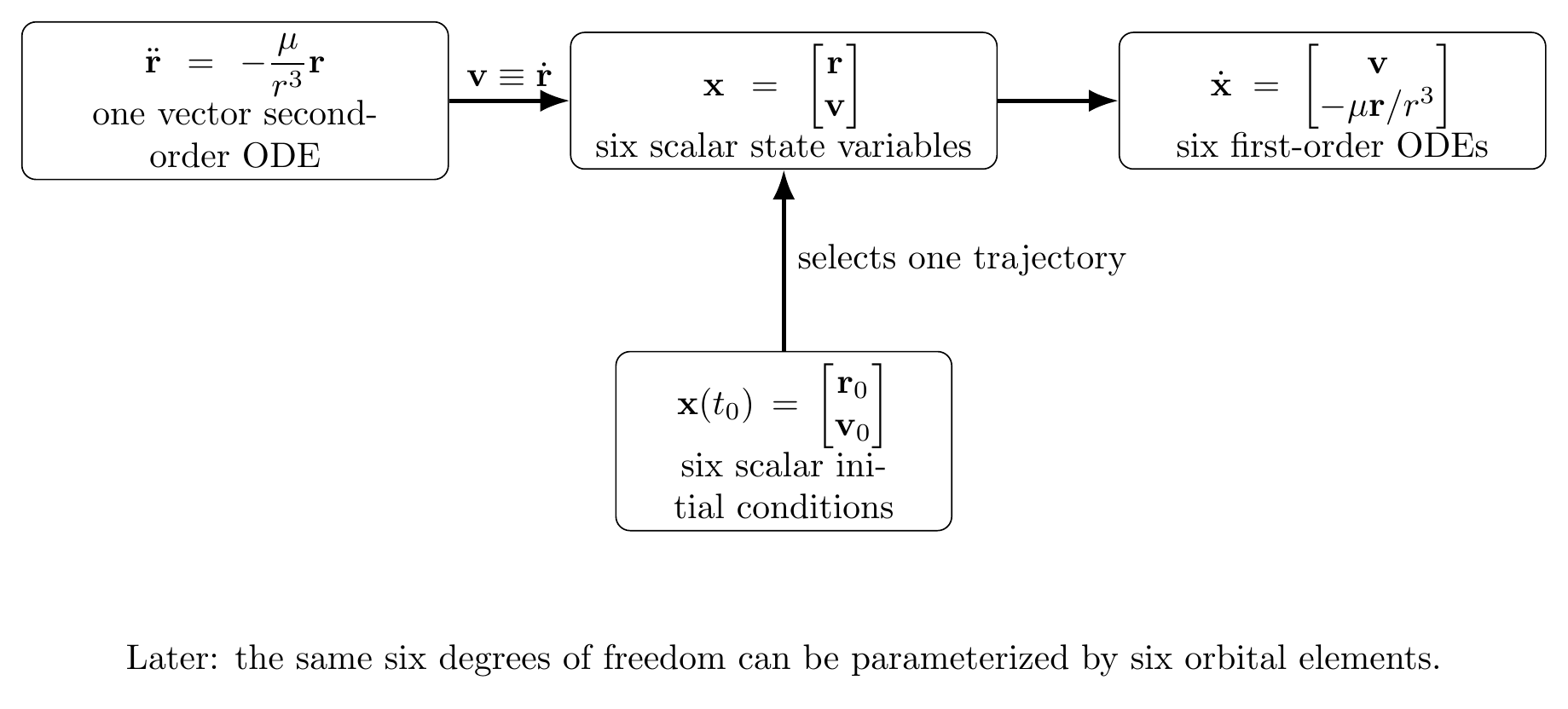
Figure 4. Conversion of the second-order vector equation into the six-state first-order form used
for propagation.
A single trajectory is selected by specifying
This requires six scalar initial values. GPSORB02 will examine carefully why those six degrees
of freedom can instead be represented by six constants such as the classical orbital
elements.
13 A first circular-orbit sanity check
The full solution of Eq. (25) is deferred until later articles, but a circular orbit provides an
immediate physical check.
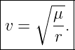
For uniform circular motion of radius r, the required inward centripetal acceleration
is
Gravity provides the inward acceleration
Equating them,
so
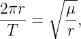
Because v = 2πr∕T,
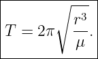
and therefore
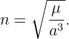
This is the circular-orbit form of Kepler’s third law and previews the mean-motion relation that
will later become
14 GPS-scale numerical check
Take a representative GPS orbital radius or semimajor axis
and the legacy GPS user-model gravitational parameter
The central gravitational acceleration magnitude is
| |ag| | =  , , | (75)
|
| ≈ 0.565 m∕s2. | (76) |
This is much smaller than surface gravity because a GPS satellite is several Earth radii from
Earth’s center.
For a circular orbit at the same radius, Eq. (69) gives
and Eq. (71) gives
These familiar GPS-scale numbers emerge directly from the same equation of motion that will later
generate the orbital-element and broadcast-ephemeris equations.
15 What is hidden inside the phrase “two-body problem”?
Equation (25) is powerful precisely because it removes many physical effects. The assumptions
should be explicit.
| Assumption | Consequence |
| Newtonian mechanics | Relativistic corrections are neglected in the basic orbit
equation. |
| Only two gravitating
bodies | Solar,
lunar, planetary, and other third-body accelerations are
absent. |
| Spherical or point-mass
Earth | Oblateness and higher gravity harmonics such as J2 are
absent. |
| Constant masses | No mass loss or thrust-driven mass variation is modeled. |
| No non-gravitational
forces | Solar radiation pressure, atmospheric drag, antenna
thrust, and maneuvers are absent. |
| Nonrotating axes for the
simple form | No Coriolis or centrifugal coordinate terms appear in
Eq. (25). |
| Earth-satellite mass ratio
m ≪ M | G(M + m) is replaced by GM to excellent accuracy. |
These are not defects. They are deliberate model reductions. The central two-body solution
provides the zeroth-order orbit around which higher-fidelity effects can be understood as
perturbations.
16 A hierarchy of orbit models
It is useful to see where Eq. (25) sits in a realistic navigation force model. One may write
schematically
The first term is
Every later term describes a departure from the ideal two-body model. The GPS control segment
may use a much higher-fidelity force model to estimate and predict the spacecraft trajectory, while
the broadcast navigation message provides users with a compact fitted representation suitable for
receiver computation.
The present article therefore supplies the physical baseline from which “perturbation” has
meaning: a perturbation is a correction to an already understood central two-body
motion.
17 Why the equation is nonlinear but highly structured
The acceleration is nonlinear because
Nevertheless, the force has two special properties:
-
1.
- it is central, because a is always parallel or antiparallel to r;
-
2.
- it is conservative, because it derives from the scalar potential −μ∕r.
Those two properties create the conserved quantities that make the two-body problem analytically
solvable. In later articles they will lead to
conservation of specific mechanical energy,
and the eccentricity vector. Together these reveal that the trajectory is a conic section and allow
the Cartesian state to be replaced by orbital elements.
We intentionally stop short of deriving those integrals here. GPSORB02 will first clarify what
“six constants” means mathematically, and GPSORB03–GPSORB04 will derive the
angular-momentum, energy, and eccentricity invariants in detail.
18 A useful linearization preview: the gravity-gradient matrix
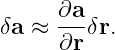
Although the exact two-body dynamics are nonlinear, navigation and estimation often need a local
linear approximation. Let
For a small position perturbation δr,
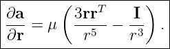
The Jacobian is
This is the point-mass gravity-gradient or tidal matrix. It is not needed yet to derive the orbit, but
it is a direct descendant of Eq. (25) and later appears naturally in variational equations,
covariance propagation, and inertial-navigation error dynamics.
18.1 Derivation of the Jacobian
Write the ith component as
Then
 | = −μ![[ ]
-∂ri −3 ∂r−3-
∂rj r + ri∂rj](https://images.physicslibrary.org/cache/objects/1258/make4ht/NewtonianTwoBodyDynamicsDerivingTheSatelliteEquationOfMotion94x.png) , , | (88)
|
| = −μ![[ − 3 −5]
δijr − 3rirjr](https://images.physicslibrary.org/cache/objects/1258/make4ht/NewtonianTwoBodyDynamicsDerivingTheSatelliteEquationOfMotion95x.png) , , | (89)
|
| = μ![[ 3rirj δij]
--5--− -3-
r r](https://images.physicslibrary.org/cache/objects/1258/make4ht/NewtonianTwoBodyDynamicsDerivingTheSatelliteEquationOfMotion96x.png) . . | (90) |
Collecting the components gives Eq. (86).
This preview reinforces an important theme of the series: once the physics is written carefully in
vector form, many later navigation equations are obtained by systematic calculus rather than by
memorizing isolated formulas.
19 From GPSORB01 to GPSORB02
We can now state precisely what Kaplan’s compact equation means:
is the relative, central, Newtonian acceleration of an ideal two-body Earth-satellite system,
normally written with μ ≈ GME and expressed in nonrotating axes. The factor r−3r is
simply the inverse-square magnitude multiplied by the radial direction. The equation may
be written as three coupled second-order scalar equations or as six first-order state
equations.
The next question is no longer “where does the force law come from?” It is:
Why does solving this three-dimensional second-order system require six
independent constants, and how can those six constants be reorganized into
quantities with direct orbital meaning?
That is the subject of GPSORB02.
References
References
[1] E. D. Kaplan and C. J. Hegarty, editors, Understanding GPS: Principles and
Applications, 2nd ed., Artech House, 2006.
[2] R. R. Bate, D. D. Mueller, and J. E. White, Fundamentals of Astrodynamics, Dover
Publications, 1971.
[3] D. A. Vallado, Fundamentals of Astrodynamics and Applications, 4th ed., Microcosm
Press, 2013.
[4] O. Montenbruck and E. Gill, Satellite Orbits: Models, Methods, and Applications,
Springer, 2000.
[5] P. D. Groves, Principles of GNSS, Inertial, and Multisensor Integrated Navigation
Systems, 2nd ed., Artech House, 2013.
[6] Global Positioning Systems Directorate, IS-GPS-200N: NAVSTAR GPS Space
Segment/Navigation User Interfaces, 1 August 2022.











![m3
[μ] = -2-.
s](https://images.physicslibrary.org/cache/objects/1258/make4ht/NewtonianTwoBodyDynamicsDerivingTheSatelliteEquationOfMotion42x.png)
![[ r] m 1
-3 = -3-= --2.
r m m](https://images.physicslibrary.org/cache/objects/1258/make4ht/NewtonianTwoBodyDynamicsDerivingTheSatelliteEquationOfMotion43x.png)
![[ ]
r- m3--1- m-
μ r3 = s2 m2 = s2 ,](https://images.physicslibrary.org/cache/objects/1258/make4ht/NewtonianTwoBodyDynamicsDerivingTheSatelliteEquationOfMotion44x.png)



![|----[-]---------------------------|
| r [ ]T |
x = v = x y z vx vy vz .|
------------------------------------](https://images.physicslibrary.org/cache/objects/1258/make4ht/NewtonianTwoBodyDynamicsDerivingTheSatelliteEquationOfMotion60x.png)
![|----[--------]--|
| v |
|˙x = − μr ∕r3 .|
-----------------|](https://images.physicslibrary.org/cache/objects/1258/make4ht/NewtonianTwoBodyDynamicsDerivingTheSatelliteEquationOfMotion61x.png)
![|--------[--]--|
| r0 |
|x(t0) = v0 .|
---------------](https://images.physicslibrary.org/cache/objects/1258/make4ht/NewtonianTwoBodyDynamicsDerivingTheSatelliteEquationOfMotion71x.png)