1 The question this series will answer
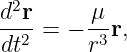
Kaplan and Hegarty introduce the ideal two-body equation of motion in the form
where
Equation (1) looks compact. The GPS broadcast ephemeris algorithm does not. A receiver
encounters quantities such as
and the six harmonic coefficients
It then performs a sequence involving mean anomaly, eccentric anomaly, true anomaly, argument of
latitude, harmonic corrections, orbital-plane coordinates, and a final transformation to Earth-fixed
coordinates.
The central question of this series is therefore
The complete conceptual path is shown in Figure 1.
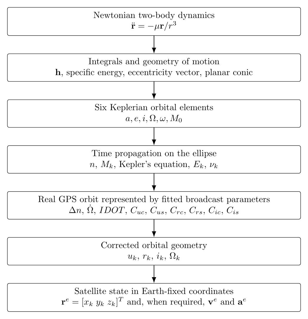
Figure 1. The central derivation path for the GPS Orbit mechanics series.
2 Start one step before Kaplan’s equation
The two-body equation is itself a consequence of Newton’s law of universal gravitation. If an
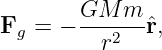
Earth of mass M attracts a satellite of mass m, the gravitational force on the satellite
is
where
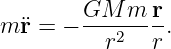
Using Newton’s second law,
gives
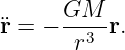
The satellite mass cancels:
Defining
produces Eq. (1).
This cancellation is physically important. In the ideal Newtonian two-body model, the orbital
acceleration of a satellite is independent of its own mass. A one-kilogram test mass and a
GPS spacecraft placed at the same position with the same velocity follow the same
trajectory.
3 Why does a three-dimensional orbit require six constants?
A common sentence in orbital mechanics is that the two-body solution contains “six constants of
integration” or “six integrals of motion.” Before deriving them, it is useful to understand why the
number six must appear.
Write Eq. (1) in Cartesian components:
| ẍ | = −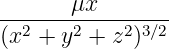 , , | (12)
|
| ÿ | = −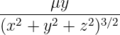 , , | (13)
|
| z | = −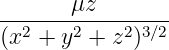 . . | (14) |
These are three coupled second-order differential equations. Equivalently, define the
six-dimensional state
Then the dynamics become six first-order differential equations,
A unique trajectory is selected by six independent scalar initial conditions, for example
This is the simplest reason that a general three-dimensional orbit needs six independent
parameters. The classical orbital elements provide a more geometrically meaningful set of six
numbers describing the same solution.
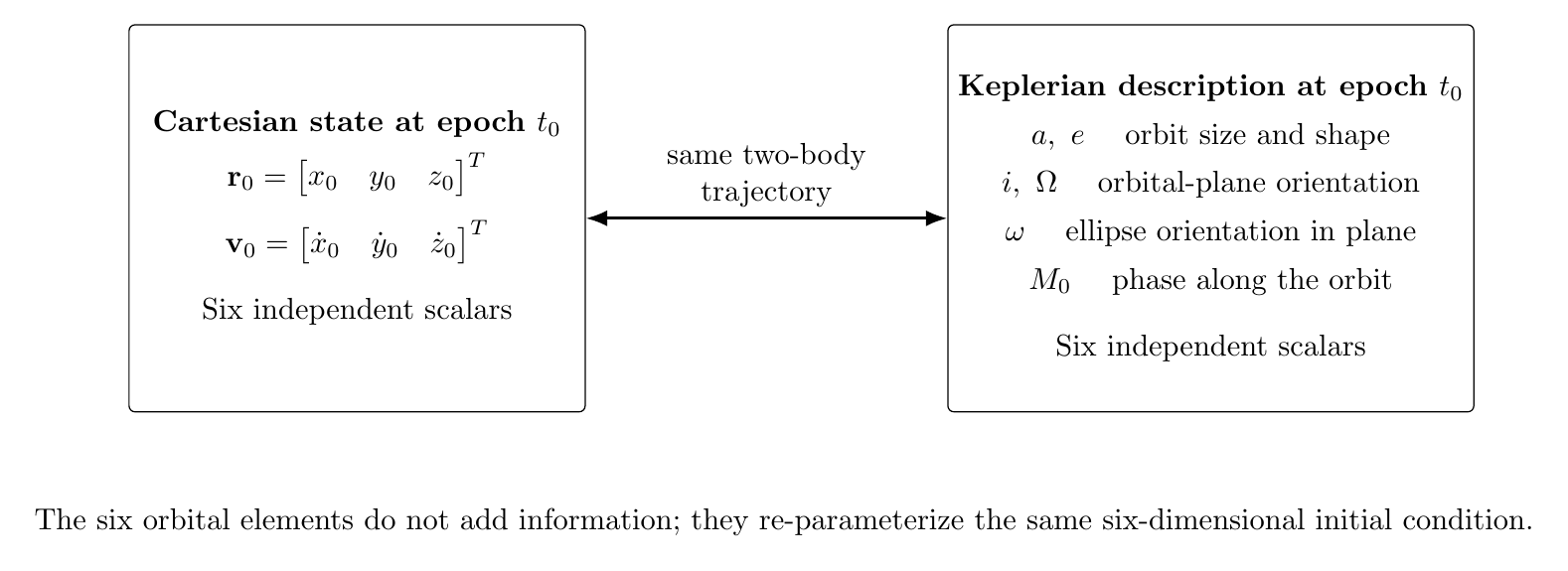
Figure 2. Cartesian initial conditions and Keplerian orbital elements are two parameterizations of
the same ideal two-body trajectory.
3.1 A terminology warning: constants of integration versus conserved quantities
The phrase “six integrals of motion” can be confusing. It does not mean that one simply writes
down six unrelated scalar conservation laws. The two-body problem contains vector invariants such
as angular momentum and the eccentricity vector, but their components are constrained and are
not all independent. The clean statement for this series is:
The general three-dimensional solution of the two-body equations contains six
independent constants. Those six degrees of freedom can be represented by a
Cartesian state at an epoch or by six orbital elements.
Later lessons will derive the useful conserved quantities and show exactly how they lead to the
conic orbit and the classical elements.
4 The first physical integral: angular momentum
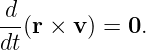
The acceleration in Eq. (1) is always parallel to r. Therefore the torque per unit mass about
Earth’s center is zero:
Using
we obtain
Hence the specific angular momentum vector
is constant in the ideal two-body problem.
This immediately establishes a major geometric fact: because both r and v remain perpendicular
to the fixed vector h, the trajectory remains in one fixed plane through the attracting
center. The three-dimensional problem has therefore acquired a two-dimensional orbital
plane.
GPSORB03 will develop this result in detail.
5 Energy gives the size of the orbit
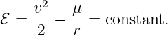
Taking the scalar product of Eq. (1) with v leads to conservation of specific mechanical
energy,
For an elliptic orbit this constant is related to the semimajor axis by
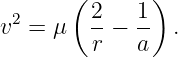
Equation (23) is the origin of the first classical orbital element, a. It is also the basis of the vis-viva
relation,
GPSORB04 will derive these equations rather than assume them.
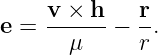
6 The eccentricity vector gives shape and periapsis direction
Another invariant of the ideal two-body problem is the eccentricity vector,
Its magnitude
is the orbital eccentricity, and its direction points toward periapsis.
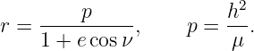
Combining h and e leads to the polar equation of a conic,
For an ellipse,
Thus Newton’s vector differential equation produces an ellipse without inserting an ellipse by
assumption.
This is one of the main derivations of the series: Newtonian dynamics → conserved quantities →
conic geometry.
7 The six classical orbital elements
For an elliptic orbit, a convenient set of six independent parameters is
Their roles separate naturally:
| Element | Physical role |
| a | Semimajor axis: sets the size and, through Kepler’s third law, the
basic orbital period. |
| e | Eccentricity: sets the shape of the conic. |
| i | Inclination: tilts the orbital plane relative to the reference
equatorial plane. |
| Ω | longitude or right ascension of the ascending node: rotates the
orbital plane about the reference z axis. |
| ω | Argument of periapsis: rotates the ellipse within its orbital plane. |
| M0 | Mean anomaly at the reference epoch: specifies where the satellite
is along the orbit at the epoch. |
For geometry, true anomaly ν0 can temporarily replace M0. For time propagation, mean anomaly
is more convenient, so GPS ultimately uses M0.
The conversion
will be derived in both directions later in the series.
8 Why three different anomalies appear
The satellite’s location along an elliptic orbit is described using three related angles.
8.1 True anomaly
The true anomaly ν is the geometrically obvious angle measured in the orbital plane
from periapsis to the satellite position vector. It appears directly in the conic equation
(27).
8.2 Eccentric anomaly
The eccentric anomaly E is an auxiliary angle associated with a circle surrounding the ellipse. It is
not merely a geometric curiosity; it provides a convenient parameterization
| xp | = a(cos E − e), | (31)
|
| yp | = a sin E. sin E. | (32) |
From this parameterization one obtains
8.3 Mean anomaly
Mean anomaly is defined so that it increases uniformly in the ideal two-body problem:
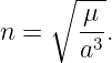
The constant rate n is the mean motion,
Kepler’s equation connects mean anomaly to eccentric anomaly:
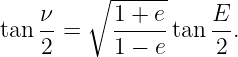
The relation between eccentric and true anomaly can be written as
These equations form the time-propagation heart of the GPS ephemeris algorithm.
GPSORB06 will derive them from area swept by the radius vector and the geometry of the
ellipse.
9 Why Kepler’s equation needs an iterative solution
Equation (36) contains E both algebraically and inside a sine function. There is no elementary
algebraic rearrangement that isolates E. A receiver therefore solves
Newton’s method uses
and gives
This is not an arbitrary numerical trick added to GPS. It follows directly from applying
Newton-Raphson iteration to Kepler’s equation. IS-GPS-200 gives this iteration explicitly in its
legacy LNAV user equations.
10 The ideal six elements are not constant for a real GPS satellite
Equation (1) treats Earth as a point mass and assumes that no other forces act. A real
satellite instead experiences a more complete acceleration model schematically represented
as
Under these perturbations, the six Keplerian parameters can still be used to describe the
instantaneous orbit, but they no longer remain exact constants.
A useful conceptual distinction is therefore
The legacy GPS broadcast quantities are Keplerian in appearance, but the control/space segment
obtains operational values by fitting the broadcast model to a propagated reference trajectory over
a finite interval. This is why it is dangerous to interpret every broadcast correction
coefficient as if it were a fundamental constant derived directly from one perturbing
force.
11 From six Keplerian elements to the broadcast ephemeris
The legacy LNAV broadcast model can be organized into three groups, as shown in Figure
2.
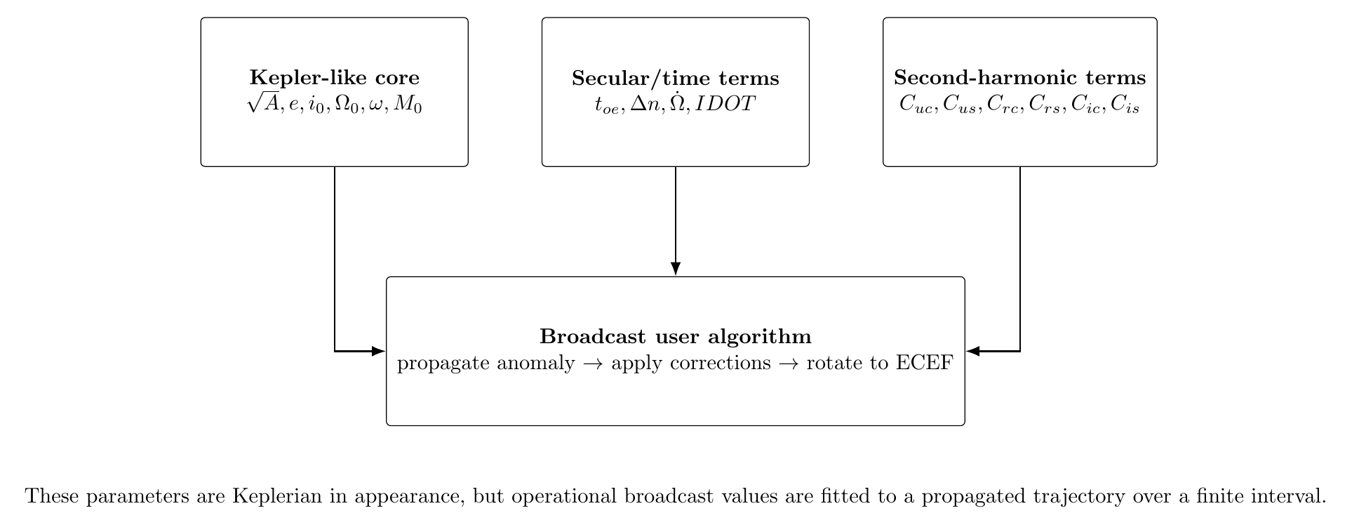
Figure 3. A useful way to organize the legacy GPS broadcast ephemeris parameters.
11.1 Kepler-like core
The core contains quantities closely associated with the six classical elements:
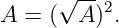
The broadcast quantity is  rather than A itself for legacy LNAV.
11.2 Reference and secular terms
The receiver also uses
Here the ephemeris reference-time parameter identifies the epoch of applicability, the mean-motion
correction modifies the nominal Keplerian mean motion, the node-rate parameter describes fitted
node evolution, and IDOT describes inclination-rate behavior.
11.3 Second-harmonic correction coefficients
Six coefficients apply periodic corrections. The pair Cuc,Cus corrects argument of latitude, Crc,Crs
corrects orbital radius, and Cic,Cis corrects inclination. The corresponding correction structure
is
The appearance of 2Φk is connected to the second-harmonic structure that naturally arises in
important nonspherical-gravity effects. Later lessons will develop that physics while keeping
separate the distinction between physical perturbation theory and the fitted coefficients actually
transmitted in the navigation message.
12 The receiver algorithm that we will derive
The legacy LNAV position algorithm can be viewed as a pipeline rather than as a collection of
unrelated formulas.
First recover the semimajor axis:
Then form the nominal mean motion
and the elapsed time from the ephemeris epoch
After the GPS-week crossover convention is applied, compute
and
Solve Kepler’s equation
for Ek, then obtain νk. Form the uncorrected argument of latitude
Apply Eq. (47), followed by
| uk | = Φk + δuk, | (55)
|
| rk | = A(1 − e cos Ek) + δrk, | (56)
|
| ik | = i0 + IDOT tk + δik. | (57) |
The in-plane coordinates become
| x′k | = rk cos uk, | (58)
|
| y′k | = rk sin uk. | (59) |
The corrected longitude of the ascending node is
where the Earth-rate quantity is the Earth rotation rate used by the GPS user algorithm.
Finally,
| xk | = x′k cos Ωk − y′k cos ik sin Ωk, | (61)
|
| yk | = x′k sin Ωk + y′k cos ik cos Ωk, | (62)
|
| zk | = y′k sin ik. | (63) |
The output is the satellite antenna phase-center position in Earth-fixed coordinates.
Every equation in this pipeline will be derived in subsequent articles.
13 Why the final coordinates are Earth-fixed
Classical orbital mechanics is most naturally developed in an inertial reference frame. GPS users,
however, need satellite positions relative to the rotating Earth. This introduces a second layer of
physics.
If an inertial frame and an Earth-fixed frame rotate relative to one another with angular velocity
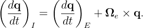
Ωe, derivatives obey
Applying this relation twice generates the familiar Coriolis and centrifugal terms. Those terms
reappear explicitly when IS-GPS-200 gives Earth-fixed satellite acceleration equations.
Thus the series begins with inertial Newtonian mechanics but ends in a rotating Earth-fixed
navigation frame. That connection is not incidental; it is the same rotating-frame physics that
appears in inertial navigation mechanization.
14 What lies beyond Kaplan’s position table
Kaplan’s Table 2.3 gives the core route to the satellite ECEF position. The current IS-GPS-200N
legacy LNAV user equations extend the chain further by presenting equations for velocity and
acceleration.
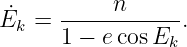
Differentiating Kepler’s equation gives
Differentiating the anomaly relationship produces the true-anomaly rate, and successive chain-rule
applications give
and eventually the Earth-fixed velocity components.
The acceleration equations bring the discussion back to force models. IS-GPS-200 includes a J2
oblateness contribution together with rotating-Earth terms. The conceptual loop of the course is
therefore
15 A GPS-scale sanity check
Before working through the full derivation, it is useful to estimate the magnitude of the quantities
involved. Take a representative GPS semimajor axis
and the GPS user value
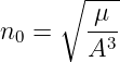
Then Eq. (35) gives approximately
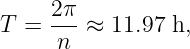
The corresponding ideal period is
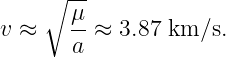
and a circular-orbit speed at this radius is approximately
These estimates will serve as useful order-of-magnitude checks in later numerical work.
16 Scope: legacy LNAV first, then modern extensions
IS-GPS-200 contains more than one navigation-message family. This series first follows the legacy
LNAV structure because it corresponds closely to Kaplan’s Table 2.3 and to the familiar
parameters  , Δn, and the six harmonic correction coefficients. In IS-GPS-200N this is the Table
20-IV family of broadcast navigation user equations.
, Δn, and the six harmonic correction coefficients. In IS-GPS-200N this is the Table
20-IV family of broadcast navigation user equations.
Modernized message structures, including the CNAV equations in the Table 30-II family, use
related mechanics but introduce different parameterizations and additional time-dependent terms.
Once the legacy derivation is complete, the modern equations can be treated as an extension rather
than mixing two parameter sets during the foundational development.
Clock correction parameters such as af0, af1, and af2 are also part of the navigation data, but they
are not orbital elements. They belong to the satellite-clock model and will be treated separately
from this orbit-mechanics sequence.
17 Series roadmap
|
|
Article |
Main objective |
|
|
|
| |
|
|
GPSORB00 |
Establish the complete path from Newton’s equation to the GPS
broadcast ephemeris and identify the physical role of every major
quantity. |
|
GPSORB01 |
Derive the two-body equation of motion from Newton’s laws and
universal gravitation; introduce inertial frames and the state-vector
formulation. |
|
GPSORB02 |
Explain rigorously why the solution requires six independent constants
and distinguish initial conditions, first integrals, and orbital elements. |
|
GPSORB03 |
Derive conservation of angular momentum, the fixed orbital plane, areal
velocity, and Kepler’s second law. |
|
GPSORB04 |
Derive specific energy, the eccentricity vector, the conic equation,
semimajor axis, eccentricity, and vis-viva equation. |
|
GPSORB05 |
Build the six classical orbital elements geometrically and derive them
from a Cartesian state. |
|
GPSORB06 |
Derive eccentric anomaly, mean anomaly, Kepler’s equation, mean
motion, and all anomaly transformations. |
|
GPSORB07 |
Derive complete state-vector-to-elements and elements-to-state-vector
transformations, including quadrant-safe implementations. |
|
GPSORB08 |
Derive the perifocal-to-inertial rotation sequence and the component
equations from rotation matrices. |
|
GPSORB09 |
Introduce the rotating Earth, inertial versus Earth-fixed coordinates,
GPS time conventions, toe, and the node-longitude equation. |
|
GPSORB10 |
Develop perturbation physics: nonspherical gravity, J2, third-body
gravity, solar radiation pressure, and osculating elements. |
|
GPSORB11 |
Explain the GPS broadcast parameterization, fitted secular terms,
and the origin and interpretation of the second-harmonic correction
structure. |
|
GPSORB12 |
Derive IS-GPS-200 Table 20-IV sheet 1 and the corresponding first part
of Kaplan Table 2.3, including Newton iteration for Kepler’s equation. |
|
GPSORB13 |
Derive Table 20-IV sheet 2 and Kaplan’s final position equations,
including the orbital-plane-to-ECEF transformation. |
|
GPSORB14 |
Derive the satellite velocity equations by differentiating the position
algorithm. |
|
GPSORB15 |
Derive the Earth-fixed acceleration equations, J2 contribution, Coriolis
term, and centrifugal term. |
|
GPSORB16 |
Carry out a complete numerical broadcast-ephemeris solution and verify
the result computationally. |
|
|
|
|
|
|
|
Separate companion articles labeled E1, E2, and so on can contain hand calculations,
MATLAB/Python exercises, and numerical verification without interrupting the main derivation
sequence.
18 Notation to keep fixed throughout the series
| Symbol | Meaning |
| r,v,a | Satellite position, velocity, and acceleration vectors. |
| r | Magnitude ∥r∥. |
| μ | Earth’s gravitational parameter used in the relevant dynamical
or GPS user model. |
| h | Specific angular momentum vector, r × v. |
| e | Eccentricity vector. |
| a,e | Semimajor axis and eccentricity. |
| i | Inclination. |
| Ω | Ascending-node angle or longitude according to the frame and
convention under discussion. |
| ω | Argument of periapsis. |
| M,E,ν | Mean, eccentric, and true anomalies. |
| u | Corrected argument of latitude when used in the broadcast
algorithm. |
| toe | Ephemeris reference time. |
| tk | Time measured from the ephemeris reference epoch after the
GPS week-crossover convention is applied. |
Angles will be treated in radians inside the mathematics unless a broadcast-message scaling
explicitly uses semicircles. Frame superscripts will be added whenever the frame is not obvious
from context.
19 What should be understood before moving to GPSORB01
The important result of this introductory article is not a single equation. It is the architecture of
the problem.
A satellite trajectory is fundamentally a solution of a differential equation. The three-dimensional
second-order equation requires six independent scalar conditions. Classical orbital elements
re-parameterize those six degrees of freedom in a way that exposes the geometry of the conic.
Kepler’s equation supplies the time evolution along that conic. Real GPS motion is not
exactly Keplerian, so the operational navigation message uses a fitted Kepler-like model
with secular and periodic correction parameters. The receiver evaluates that model
at the desired transmit time and finally expresses the satellite position in Earth-fixed
coordinates.
In compact form,
GPSORB01 now returns to the beginning and derives Eq. (1) carefully from Newtonian mechanics,
including the assumptions hidden inside the phrase “two-body problem.”
References
References
[1] E. D. Kaplan and C. J. Hegarty, editors, Understanding GPS: Principles and
Applications, 2nd ed., Artech House, 2006.
[2] Global Positioning Systems Directorate, IS-GPS-200N: NAVSTAR GPS Space
Segment/Navigation User Interfaces, 1 August 2022. In particular, see the legacy LNAV
ephemeris definitions and Table 20-IV broadcast navigation user equations.
[3] D. A. Vallado, Fundamentals of Astrodynamics and Applications, 4th ed., Microcosm
Press, 2013.
[4] R. R. Bate, D. D. Mueller, and J. E. White, Fundamentals of Astrodynamics, Dover
Publications, 1971.
[5] O. Montenbruck and E. Gill, Satellite Orbits: Models, Methods, and Applications,
Springer, 2000.








![[ ] [ ]
x = r = x y z ˙x y˙ z˙T .
v](https://images.physicslibrary.org/cache/objects/1255/make4ht/FromNewtonsEquationToTheGPSBroadcastEphemerisADerivationRoadmap14x.png)
![[ ]
v
˙x = 3 .
− μr ∕r](https://images.physicslibrary.org/cache/objects/1255/make4ht/FromNewtonsEquationToTheGPSBroadcastEphemerisADerivationRoadmap15x.png)