1 Where GPSORB03 fits in the derivation chain
GPSORB01 derived the ideal Earth-satellite relative equation of motion,
where  is the satellite position relative to Earth’s center,
  , and
, and  is Earth’s
gravitational parameter. GPSORB02 then explained why this three-dimensional second-order
equation requires six independent scalar constants to specify one unique orbit.
is Earth’s
gravitational parameter. GPSORB02 then explained why this three-dimensional second-order
equation requires six independent scalar constants to specify one unique orbit.
The next task is to expose some of those constants physically. The first conserved quantity to
derive is angular momentum. It is especially important because it proves that the ideal orbit is
planar before any conic-section geometry is introduced.
The chain developed here is
That last expression is Kepler’s second law in differential form.
2 Angular momentum: physical and specific forms
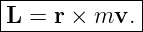
For a particle of mass  moving with position
  and velocity
  , the angular momentum
about the origin is
, the angular momentum
about the origin is
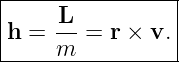
Because the satellite mass is constant, orbital mechanics usually divides by  and works with
the specific angular momentum,
and works with
the specific angular momentum,
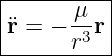
The adjective “specific” means “per unit mass.” The units are therefore
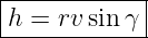
The magnitude of a cross product is
where  is the angle between
  and
and  . If
. If  denotes the velocity component perpendicular
to
denotes the velocity component perpendicular
to  , then
Thus angular momentum measures the transverse, or sideways, part of the orbital motion. Purely
radial velocity contributes no angular momentum about Earth’s center.
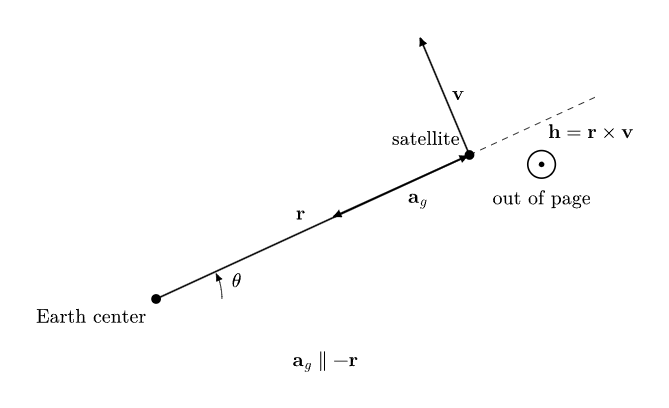
Figure 1. Central gravity is radial, while the specific angular momentum is perpendicular to the
plane containing position and velocity.
3 Why central gravity produces zero torque
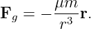
The rotational analogue of Newton’s second law is obtained from torque. The gravitational force
on a satellite of mass  is
is
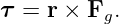
The torque about Earth’s center is
Substituting Eq. (6),
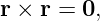
But any vector crossed with itself vanishes,
so
This is the geometric core of the result. Gravity points along the radius vector, so it has no
moment arm about Earth’s center. A radial force can change the magnitude and direction of
velocity, but it cannot exert a torque about the force center.
4 Direct derivation of conserved angular momentum
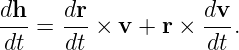
Start with the definition
Differentiate with respect to time. The cross product obeys a product rule,
Since 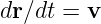 and
and 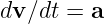 ,
,
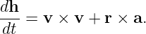
The first cross product is zero,
Using the two-body acceleration from Eq. (1),
Therefore
and hence
The word vector matters. Conservation of  means both its magnitude and its direction remain
fixed in the ideal two-body problem.
means both its magnitude and its direction remain
fixed in the ideal two-body problem.
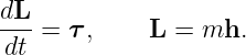
Equation (13) is equivalent to the zero-torque result because
For a constant satellite mass, zero torque implies constant  .
.
5 A subtle but powerful point: the inverse-square form was not required
The conservation proof did not actually use the  magnitude of Newtonian gravity. It used
only the fact that the acceleration is parallel or antiparallel to
magnitude of Newtonian gravity. It used
only the fact that the acceleration is parallel or antiparallel to  .
.
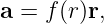
For any central-force acceleration of the form
we obtain
so
Newton’s inverse-square law is special for additional reasons: it leads to closed conic trajectories
and to another conserved vector, the eccentricity vector. But planarity and constant areal velocity
arise more generally from central-force symmetry.
6 Conservation of angular momentum proves orbital planarity
By definition,
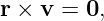
A cross product is perpendicular to both input vectors, so
At every instant, the position and velocity therefore lie in the plane perpendicular to
 .
.
Because Eq. (14) says that  is a constant vector, the orientation of this plane does not change
with time. The plane also passes through the force center because
is a constant vector, the orientation of this plane does not change
with time. The plane also passes through the force center because  is measured from Earth’s
center. Thus
is measured from Earth’s
center. Thus
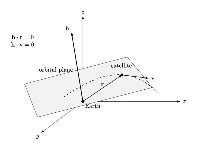
Figure 2. Position and velocity remain in the fixed orbital plane perpendicular to the conserved
angular-momentum vector.
This is a major reduction in the problem. We began with a three-dimensional vector differential
equation, yet conservation of angular momentum tells us that once the orbital plane is
known, all subsequent Keplerian motion may be analyzed in two dimensions inside that
plane.
The radial special case
If
then  . Position and velocity are parallel, so the motion is purely radial. This is a degenerate
case rather than an ordinary orbit with a well-defined orbital plane. In normal satellite motion,
. Position and velocity are parallel, so the motion is purely radial. This is a degenerate
case rather than an ordinary orbit with a well-defined orbital plane. In normal satellite motion,
 .
.
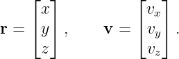
7 The angular-momentum vector in Cartesian coordinates
Let
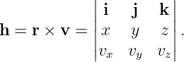
Then
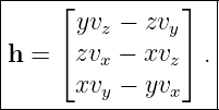
Expanding the determinant,
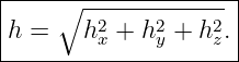
Its magnitude is
These equations are the practical bridge from a Cartesian navigation state to orbital
geometry. Given  at one epoch, computing
  immediately gives the orbital-plane
normal.
immediately gives the orbital-plane
normal.
8 A second derivation using polar coordinates
Because the motion is planar, introduce polar basis vectors  and
and  inside the orbital plane.
The position is
inside the orbital plane.
The position is
The polar basis rotates with angle  , so
, so
Differentiate Eq. (23):
The velocity therefore has a radial component
and a transverse component
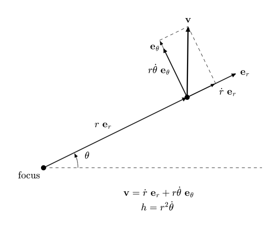
Figure 3. Polar decomposition of orbital velocity into radial and transverse components.
Now compute the specific angular momentum:
Substituting the polar forms of position and velocity gives
Expanding the cross product,
Since
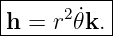
where  is the unit normal to the orbital plane,
Taking magnitudes,
This is one of the most useful identities in orbital mechanics.
9 The same result from the transverse equation of motion
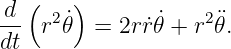
Differentiating the polar velocity gives the standard polar acceleration,
Central gravity has no transverse component, so
Multiply by  :
:
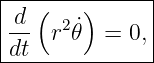
But the left-hand side is exactly
Therefore
which gives again
The vector proof and the polar-coordinate proof are the same physics expressed in two
different mathematical languages. The vector proof emphasizes zero torque and plane
orientation; the polar proof emphasizes the coupling between orbital radius and angular
rate.
10 Deriving Kepler’s second law from angular momentum
Consider the radius vector moving from  to
to  during a small time
  . The small swept
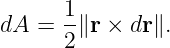
area is approximately the area of a triangle,
. The small swept
area is approximately the area of a triangle,
Because
we obtain
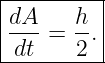
Divide by  :
:
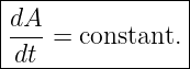
Since  is constant,
This is Kepler’s second law: the radius vector sweeps out equal areas in equal times.
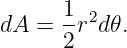
The same result follows immediately from Eq. (30). A polar area element is
Hence
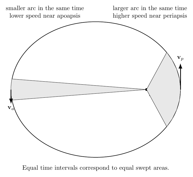
Figure 4. Equal time intervals sweep equal areas; the satellite therefore moves faster near
periapsis and slower near apoapsis.
11 Why orbital speed changes around an ellipse
Equation (5) gives
For a fixed  , the transverse speed is larger when
  is smaller and smaller when
  is
larger.
is
larger.
At periapsis and apoapsis,  is at a local minimum or maximum, so
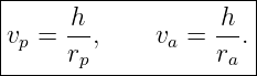
The velocity is therefore purely transverse at those two points. Thus
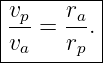
Dividing,
This result follows from angular momentum alone. Energy conservation will later supply the
absolute values of the speeds and lead to the vis-viva equation.
12 Angular rate is strongly coupled to orbital radius
From Eq. (30),
The angular rate therefore varies as  . This is stronger than the
  dependence of
transverse speed because the same angular change corresponds to a larger arc length at larger
radius.
dependence of
transverse speed because the same angular change corresponds to a larger arc length at larger
radius.
This relationship is central to later anomaly variables. True anomaly does not increase uniformly
with time on an eccentric orbit. The satellite advances rapidly in angle near periapsis and slowly
near apoapsis. The mean anomaly introduced later is useful precisely because it advances linearly
in the ideal Kepler problem.
13 The direction of angular momentum encodes the orbital plane
Let the reference  -axis be represented by the unit vector
The inclination  is the angle between
  and the positive
  -axis. Since
  is a unit vector,
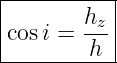
the dot product gives
is a unit vector,
the dot product gives
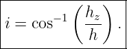
Therefore
and
The line where the orbital plane intersects the reference equatorial plane is the line of nodes. A
vector toward the ascending-node direction is
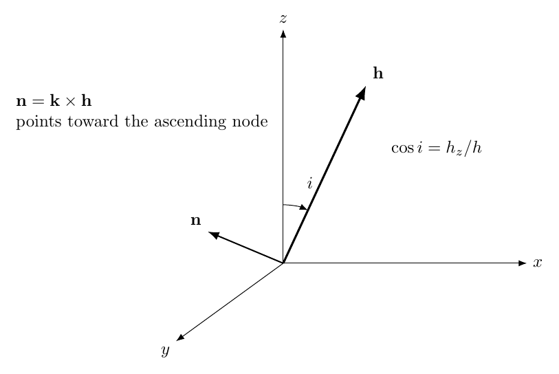
Figure 5. The angular-momentum direction determines orbital inclination, while the node vector
lies along the intersection of the orbital and reference planes.
Thus a single conserved vector already provides two of the geometric ingredients needed for the
classical orbital elements:
- its direction determines the orientation of the orbital plane;
- its angle from the reference pole determines inclination;
- together with the reference pole, it determines the node line.
The right ascension of the ascending node will be derived carefully when the full classical element
set is introduced.
14 Numerical scale for a nominal GPS orbit
Consider a nearly circular GPS-like orbit with radius
and use
For a circular orbit, radial force balance gives
so
Numerically,
Because the velocity is perpendicular to the radius in a circular orbit,
so
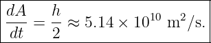
The areal velocity is therefore
The orbital angular rate is
Hence the period is approximately
This provides a useful scale check for GPS orbital mechanics.
15 What angular momentum does and does not determine
Conservation of  is extremely powerful, but it does not by itself determine the entire orbit. The
three components of
is extremely powerful, but it does not by itself determine the entire orbit. The
three components of  specify the plane orientation and the amount of transverse motion, yet
additional information is required to determine the size and shape of the conic and the satellite’s
phase on it.
specify the plane orientation and the amount of transverse motion, yet
additional information is required to determine the size and shape of the conic and the satellite’s
phase on it.
A useful summary is:
- Direction of
 : orientation of the orbital plane.
- Magnitude
 : strength of transverse motion and constant areal rate.
- Specific energy: orbit size and bound versus unbound character.
- Eccentricity vector: orbit shape and periapsis direction.
- Phase variable: location of the satellite on the conic at an epoch.
This is why GPSORB02 emphasized that the conserved vectors are constrained and should not be
counted naively as independent scalar constants.
16 What happens in the real GPS problem
The ideal result
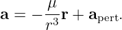
assumes a perfectly central force. Real satellite dynamics contain perturbing accelerations,
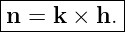
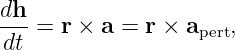
Then
so
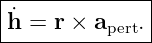
Any perturbing acceleration with a component that produces nonzero torque about Earth’s center
can change the angular-momentum vector.
For GPS satellites, important departures from the ideal central model include Earth’s nonspherical
gravity field, third-body gravity, solar radiation pressure, and other smaller effects. The most
important conceptual consequence for this article is that the orbital plane is no longer perfectly
fixed. Its orientation changes slowly, which later appears in orbital-element rates such as nodal
precession and inclination variation.
This provides a physical bridge to the extra rate parameters seen in GPS broadcast ephemerides.
The broadcast model does not discard Keplerian geometry; it augments that geometry
so a compact parameter set can track a real perturbed satellite over the intended fit
interval.
17 Connection to the next derivation
Angular momentum has reduced the three-dimensional problem to a two-dimensional one. The
next step is to determine the shape of the trajectory inside that plane.
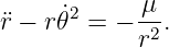
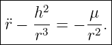
The radial equation in polar coordinates is obtained from Eq. (31):
Using
this becomes
The term
encodes the angular-motion contribution to the radial dynamics.
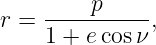
In the next stages of the series, energy conservation and the eccentricity vector will turn this radial
dynamics into the conic equation
and will establish
Those results will connect the conserved quantities derived from Newton’s law to semimajor axis,
eccentricity, periapsis, and ultimately the six orbital elements used as the foundation of GPS
ephemeris models.
Key results
The principal results of this article are
Together they establish the most important geometric consequence of a central gravitational
force:
References
[1] E. D. Kaplan and C. J. Hegarty, editors, Understanding GPS/GNSS: Principles and
Applications, 3rd ed., Artech House, 2017.
[2] D. A. Vallado, Fundamentals of Astrodynamics and Applications, 4th ed., Microcosm
Press, 2013.
[3] H. D. Curtis, Orbital Mechanics for Engineering Students, 4th ed.,
Butterworth-Heinemann, 2020.
[4] R. H. Battin, An Introduction to the Mathematics and Methods of Astrodynamics,
Revised ed., AIAA, 1999.
[5] H. Goldstein, C. Poole, and J. Safko, Classical Mechanics, 3rd ed., Addison-Wesley,
2001.


![m2-
[h] = s .](https://images.physicslibrary.org/cache/objects/1257/make4ht/AngularMomentumOrbitalPlanarityAndKeplersSecondLaw11x.png)