1 Why GPSORB07 belongs between time propagation and frame rotation
GPSORB06 ended with a complete phase-propagation chain for an ideal ellipse,
At that stage the semimajor axis a, eccentricity e, and true anomaly ν determine where the
satellite lies on the conic, but we have not yet written its Cartesian position and velocity in the
orbital plane.
GPSORB08 will rotate an orbital-plane state into an Earth-centered inertial frame using Ω, i, and
ω. Therefore the missing bridge is
before any three-dimensional orientation transformation is applied.
This separation is conceptually useful. The elements a, e, and ν describe the instantaneous
geometry and motion within the orbital plane. The elements Ω, i, and ω describe how that plane is
oriented relative to an external reference frame. The PQW frame isolates the first problem from
the second.
2 The perifocal frame
The perifocal frame is an orthonormal right-handed frame attached to the Keplerian orbit. Its
basis vectors are
They are defined geometrically:
- P points from the occupied focus toward periapsis.
- Q lies in the orbital plane, 90∘ ahead of P in the direction of increasing true anomaly.
- W = h is normal to the orbital plane and points along the specific angular-momentum
vector.
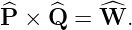
Thus
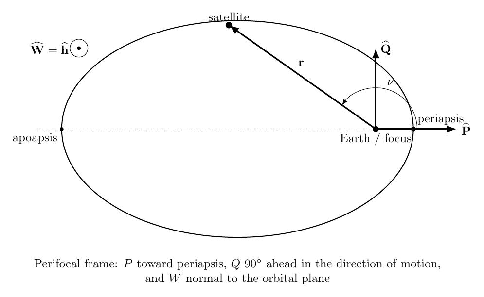
Figure 1. The perifocal frame is built directly from the orbit: P points toward periapsis, Q lies 90
degrees ahead in the direction of motion, and W is normal to the plane.
In this frame, true anomaly ν is especially simple: it is the angle measured from the positive P axis
to the radius vector. Therefore the orbital geometry itself supplies the polar coordinate
system.
3 The three scalar quantities needed first
Before writing the Cartesian state, compute three familiar orbital quantities.
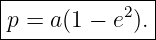
The semilatus rectum is
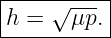
From GPSORB03 and GPSORB04,
so the magnitude of the specific angular momentum is
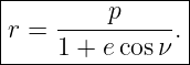
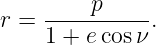
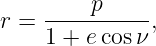
Finally, the conic-orbit equation is
Equations (5)–(8) already contain nearly everything required for the orbital-plane state. The
remaining work is to express the local radial and transverse directions in the fixed PQW basis and
then derive the corresponding velocity components.
4 Radial and transverse unit vectors
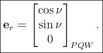
Because ν is measured from the P axis, the radial unit vector is
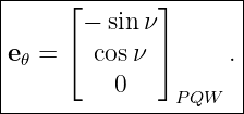
The transverse unit vector points 90∘ ahead in the direction of increasing ν,
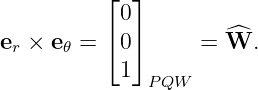
These satisfy
and
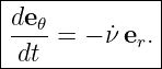
Differentiating Eq. (9) with respect to ν gives
so by the chain rule
Similarly,
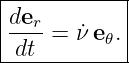
These moving-basis derivatives are the essential kinematic fact behind the orbital velocity
formula.
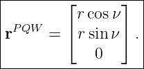
5 Position in the PQW frame
The position vector is simply
Substituting Eq. (9),
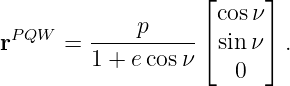
Using Eq. (8), this can also be written
This is the first half of the perifocal state. The third component vanishes because the PQ plane is
the orbital plane.
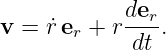
6 Velocity in polar form
Differentiate
The product rule gives
Using Eq. (14),
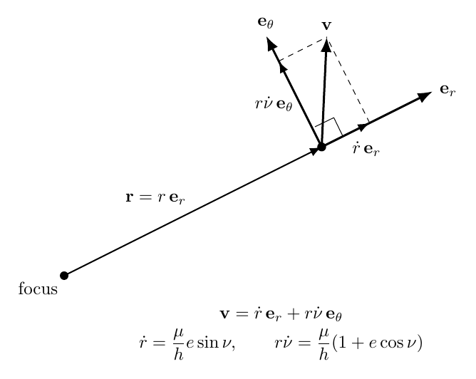
Figure 2. Orbital velocity separates naturally into radial and transverse components in the
instantaneous polar basis.
The first term changes the orbital radius. The second term sweeps the radius vector around the
focus. A circular orbit has zero radial rate, but an eccentric orbit generally has both
terms.
7 Deriving the radial speed
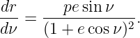
Start with the conic equation,
Differentiate with respect to ν:
From angular-momentum conservation,
so
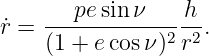
The chain rule gives
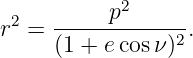
Substitute Eqs. (23) and (25):
But Eq. (8) implies
Therefore
Using p = h2∕μ,
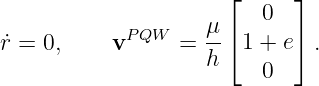
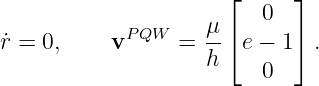
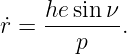
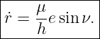
This formula immediately gives several physical checks. At periapsis, ν = 0, so the radial rate
vanishes. At apoapsis, ν = π, so the radial rate vanishes again. Between periapsis and apoapsis,
0 < ν < π and the radial rate is positive: the satellite moves outward. On the return half of the
orbit, sin ν < 0 and the satellite moves inward.
8 Deriving the transverse speed
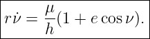
The transverse speed is the second scalar in Eq. (21),
Using the angular-momentum relation from Eq. (25),
Now substitute Eq. (8):
Again using p = h2∕μ,
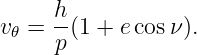
Unlike the radial component, the transverse component does not vanish at periapsis or apoapsis.
Indeed, at periapsis it is largest because the orbital radius is smallest while the angular momentum
is fixed.
9 Assembling the compact perifocal velocity vector
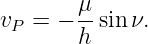
Insert Eqs. (30) and (34) into Eq. (21):
Now substitute the two unit vectors from Eqs. (9) and (10). The P component becomes
The two mixed terms cancel, leaving
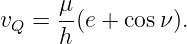
The Q component becomes
Use sin 2ν + cos 2ν = 1 to obtain
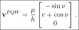
Therefore
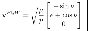
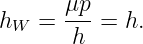
Because h =  ,
,
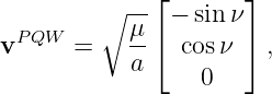
This is the standard perifocal velocity formula. The derivation shows exactly where each term
comes from: the − sin ν term emerges from cancellation between radial and transverse
motion, while the e + cos ν term contains both the circular part and the eccentricity
correction.
10 The whole state reconstruction in one chain
For implementation, the minimum sequence is
followed by Eqs. (17) and (40). No node angle, inclination, or argument of periapsis is needed yet
because the result is still expressed in the orbit’s own PQW coordinates.
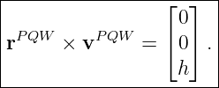
11 Check 1: the cross product must reproduce angular momentum
A strong verification is
Using Eqs. (17) and (40), only the W component survives:
Collect terms:
Thus
Since r(1 + e cos ν) = p,
Therefore
The reconstructed state has exactly the angular momentum used to build it.
12 Check 2: recovering the vis-viva equation
Square Eq. (41):
Expand the bracket:
Hence
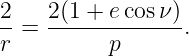
From r = p∕(1 + e cos ν),
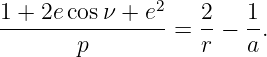
Using p = a(1 − e2), one can verify that
Therefore Eq. (53) becomes
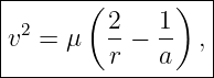
which is the vis-viva equation derived in GPSORB04. The vector reconstruction and the scalar
energy relation are therefore consistent.
13 Flight-path angle
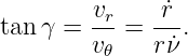
The velocity vector is not generally perpendicular to the radius vector. Define the flight-path angle
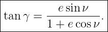
γ as the angle from the local transverse direction toward the velocity vector. Then
Substituting Eqs. (30) and (34) gives
For a circular orbit, e = 0 and therefore γ = 0 everywhere: velocity is exactly transverse. For an
eccentric ellipse, γ = 0 at periapsis and apoapsis but is nonzero elsewhere. This is the precise
mathematical version of the statement that the velocity vector is tangent to the orbital trajectory
but is not generally perpendicular to the radius vector.
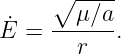
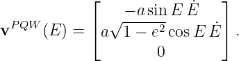
14 An equivalent reconstruction using eccentric anomaly
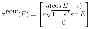
GPSORB06 derived the focus-centered ellipse coordinates
Therefore the perifocal position can be written directly as
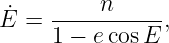
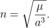
Kepler’s equation gives
where
Because
we can rewrite the eccentric-anomaly rate as
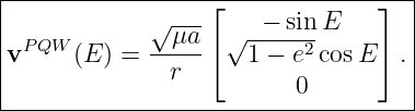
Differentiate Eq. (61):
Substitution gives
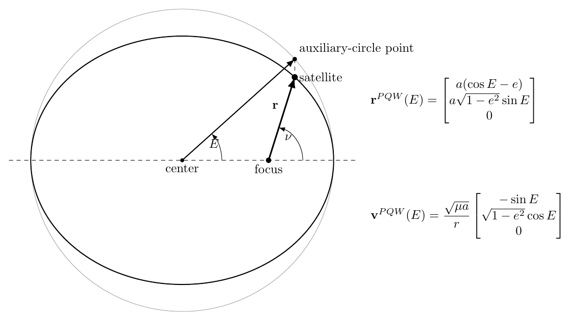
Figure 3. The same perifocal state can be reconstructed from eccentric anomaly E or true
anomaly nu.
Equations (61) and (67) are especially convenient when Kepler’s equation has just been solved
numerically for E. The true-anomaly formulas and eccentric-anomaly formulas must produce the
same state to numerical precision.
15 Worked GPS-like example
Use the same idealized orbit employed in GPSORB05 and GPSORB08,
with
First compute the semilatus rectum:
Then
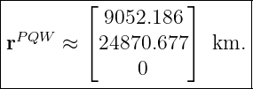
The orbital radius is
The position vector is therefore
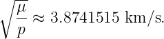
The velocity scale is
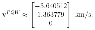
Thus
The radial and transverse components are
Thus most of the velocity is transverse, but the nonzero positive radial component shows that the
satellite is moving outward at ν = 70∘.
The total speed is
The specific mechanical energy computed from the reconstructed state is
which agrees with
For an independent anomaly check, the corresponding eccentric anomaly is
Using Eqs. (61) and (67) reproduces the same position and velocity components shown
above.
16 Important limiting cases
16.1 Circular orbit
If e = 0, then
The velocity becomes
which is exactly perpendicular to the radius vector.
The caveat is geometric: in a perfectly circular orbit, periapsis is undefined, so the P axis itself is
not unique. One may choose a convenient in-plane reference direction and use argument of latitude
instead. The state remains perfectly well defined even though the classical periapsis-based
coordinates become singular.
16.2 Periapsis and apoapsis
At periapsis, ν = 0, so
At apoapsis, ν = π, so
The negative Q component at apoapsis is not a contradiction: at ν = π, the local transverse
direction points in the negative P-frame Q sense associated with the instantaneous geometry of the
position angle. The vector remains tangent to the orbit and consistent with increasing
ν.
17 A compact implementation recipe
Given a, e, ν, and μ for a nonsingular Keplerian ellipse:
-
1.
- Compute p = a(1 − e2).
-
2.
- Compute h =
 .
.
-
3.
- Compute r = p∕(1 + e cos ν).
-
4.
- Form rPQW = [r cos ν, r sin ν, 0]T .
-
5.
- Form vPQW =
 [− sin ν, e + cos ν, 0]T .
-
6.
- Verify ∥r × v∥ = h and v2 = μ(2∕r − 1∕a).
If the propagator naturally produces E first, Eqs. (61) and (67) provide an equally
valid route. Comparing the E-based and ν-based states is an excellent software unit
test.
18 Bridge to GPSORB08
GPSORB07 has deliberately stopped before applying the three orientation elements. The state
currently has the form
These vectors describe the full instantaneous motion in the orbital plane, but they do not yet tell
us how that plane sits in inertial space.
GPSORB08 supplies the missing transformation,
where
Thus the clean conceptual sequence is
GPSORB06 supplied the clock, GPSORB07 supplies the orbital-plane state, and GPSORB08
supplies the three-dimensional orientation.
References
References
[1] E. D. Kaplan and C. J. Hegarty, eds., Understanding GPS/GNSS: Principles and
Applications, 3rd ed., Artech House.
[2] D. A. Vallado, Fundamentals of Astrodynamics and Applications, 4th ed., Microcosm
Press.
[3] H. D. Curtis, Orbital Mechanics for Engineering Students, Elsevier.
[4] R. R. Bate, D. D. Mueller, and J. E. White, Fundamentals of Astrodynamics, Dover
Publications.
[5] Global Positioning Systems Directorate, IS-GPS-200, Navstar GPS Space Segment /
Navigation User Segment Interfaces.














![μ
v = --[esin ν er + (1 + ecos ν)e𝜃].
h](https://images.physicslibrary.org/cache/objects/1265/make4ht/PerifocalStateVectorsReconstructingPositionAndVelocityFromOrbitalElements34x.png)
![μ
--[e sin ν cos ν − (1 + ecosν )sin ν].
h](https://images.physicslibrary.org/cache/objects/1265/make4ht/PerifocalStateVectorsReconstructingPositionAndVelocityFromOrbitalElements35x.png)
![μ [ ]
-- e sin2 ν + (1 + e cosν) cosν .
h](https://images.physicslibrary.org/cache/objects/1265/make4ht/PerifocalStateVectorsReconstructingPositionAndVelocityFromOrbitalElements37x.png)






![v2 = μ-[sin2ν + (e + cosν )2] .
p](https://images.physicslibrary.org/cache/objects/1265/make4ht/PerifocalStateVectorsReconstructingPositionAndVelocityFromOrbitalElements51x.png)