The Physical Structure of Classical Electrodynamics

(Topic)

ED01: The Physical Structure of Classical Electrodynamics

Classical electrodynamics is a theory of charged matter interacting through electric and magnetic fields.

The subject is often introduced as a collection of formulas: Coulomb’s law, Gauss’s Law, the Biot-Savart law, Faraday induction, Ampere’s law, Maxwell’s correction, electromagnetic waves, and the Lorentz force. Those formulas become much easier to organize once the underlying structure of the theory is made explicit.

At the broadest level, classical electrodynamics contains three kinds of objects:

sources, such as charge and current distributions;
fields, principally E and B;
responses, such as forces, accelerations, work, energy transfer, and measured voltages or currents.

The central chain is therefore

sources −→ electromagnetic fields −→ motion and measurable response.

(1)

In a fully self-consistent problem, the chain closes back on itself because charged matter moves, moving charge changes the current distribution, and the changed sources alter the fields.

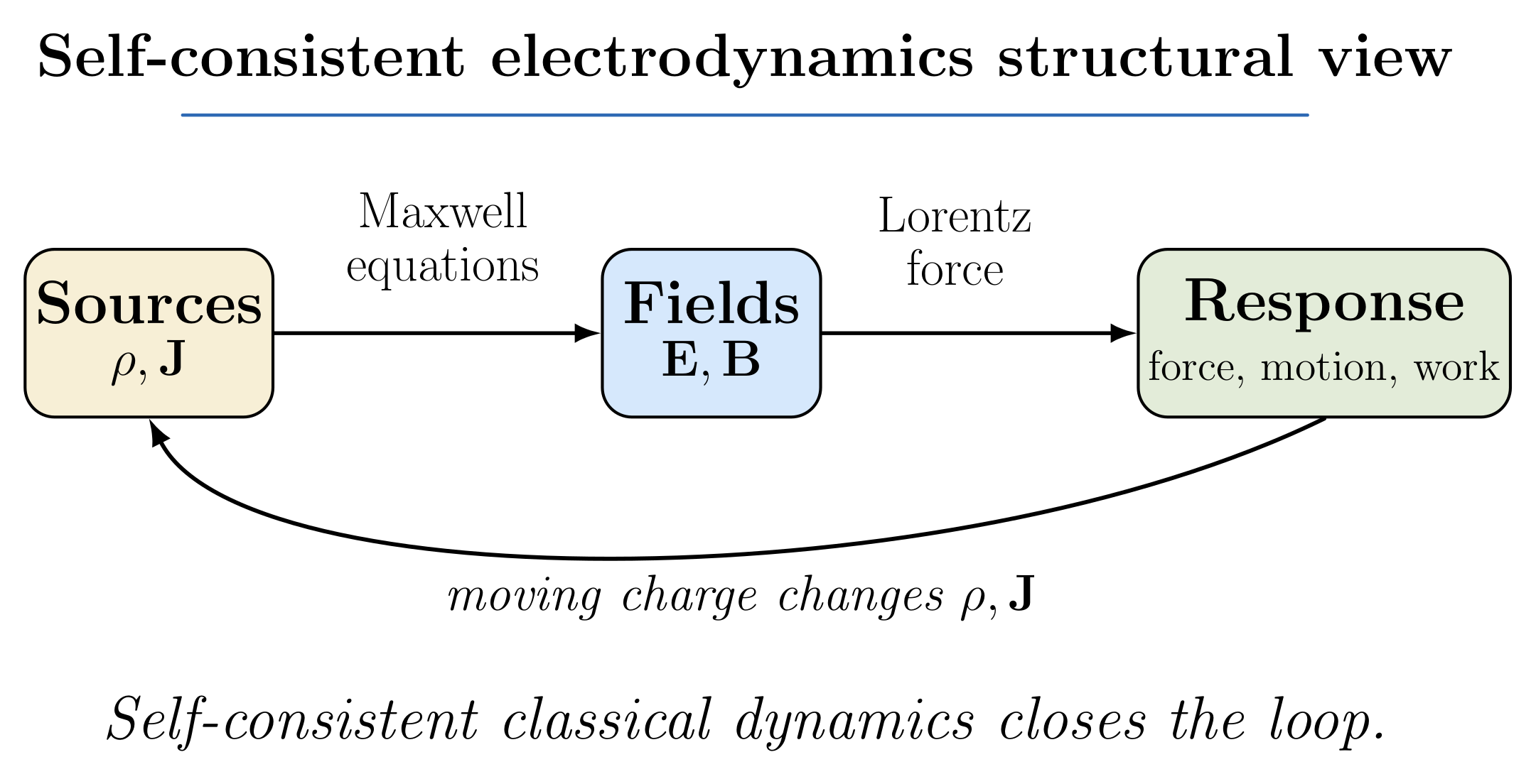
Figure 1. Structural view of classical electrodynamics. Charge density ρ and current density J act as sources for the electromagnetic fields. The fields act on charged matter through the Lorentz force. Motion of that matter can then change the sources, closing the dynamical loop.

This article establishes that structure before the ED series begins deriving the individual laws in detail.

1 The physical objects of the theory

A useful way to organize electrodynamics is to separate the description of matter from the description of the electromagnetic field.

A point particle may be characterized by quantities such as

q, m, r(t), v(t).

(2)

Here q is electric charge, m is mass, r(t) is position, and

dr v(t) = --- dt

(3)

is velocity.

A continuous distribution of charged matter is described more naturally by fields such as

ρ(r,t)

(4)

and

J (r,t),

(5)

where ρ is charge density and J is current density.

The electromagnetic state is described by two vector fields,

E (r,t)

(6)

and

B (r,t).

(7)

The notation already tells us something important. A particle position is one vector that changes with time. A field assigns a vector to every spatial point and, in general, to every time.

Thus

E (r,t)

(8)

means that the Electric Field may be different at different positions and may also change with time.

2 Point sources and continuous sources

Introductory mechanics often begins with particles. Electrodynamics uses both particle and continuum descriptions.

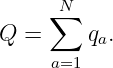
For discrete point charges,

q1,q2,...,qN,

(9)

the total charge is

∑N Q = qa. a=1

(10)

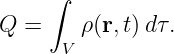
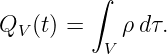
For a continuous charge distribution, the corresponding description is

dq = ρ(r,t)dτ,

(11)

where dτ is an element of volume.

Therefore

∫ Q = ρ(r,t)dτ. V

(12)

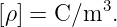
The units are

3 [ρ ] = C ∕m .

(13)

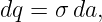
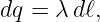
Surface and line distributions are also useful:

dq = σ da,

(14)

dq = λ dℓ,

(15)

with

2 [σ] = C∕m , [λ] = C ∕m.

(16)

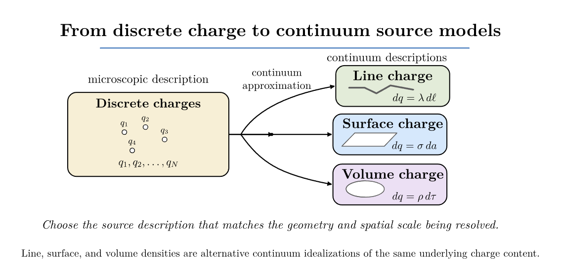
Figure 2. The same physical charge can be modeled at different levels. Discrete point charges are useful when individual particles matter. Charge density ρ(r,t) is useful when many charges can be represented as a continuum. Surface density σ and line density λ are lower-dimensional idealizations.

3 Current density

Charge density tells us where charge is. Current density tells us how charge is moving through space.

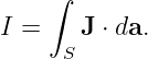
Consider a small oriented surface element

da.

(17)

The current through that surface is defined by

∫ I = J ⋅ da. S

(18)

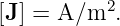
Thus the units of current density are

[J ] = A ∕m2.

(19)

For a simple continuum with charge density ρ moving with local velocity u,

J = ρu.

(20)

Equation (20) is not the most general microscopic description of all conducting matter, but it captures the basic connection between moving charge and current density.

The distinction between ρ and J will be central throughout the ED series:

static charge density is associated with electrostatic fields;
steady current density is associated with magnetostatic fields;
time-dependent ρ and J require the full dynamical electromagnetic theory.

4 Charge conservation

Charge is conserved. Charge cannot disappear from a region unless it flows out through the region’s boundary, and it cannot appear unless charge flows in.

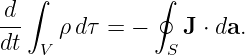
For a fixed volume V bounded by a closed surface S,

∫ Q (t) = ρ dτ. V V

(21)

If outward current through the boundary is positive, charge inside the volume decreases:

∫ ∮ d -- ρdτ = − J ⋅ da. dt V S

(22)

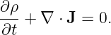
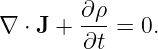
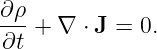
Using the divergence theorem later gives the local continuity equation

∂ρ ---+ ∇ ⋅ J = 0. ∂t

(23)

We will derive and use this relation repeatedly later. For now its physical meaning is more important than its mathematical form: local charge density can change only if current has nonzero net flow into or out of the neighborhood.

5 What is an electromagnetic field?

A field is not merely a bookkeeping device for force at a distance. In classical electrodynamics, the field is part of the physical state of the system.

The electric field is a vector field

E (r,t),

(24)

and the magnetic field is a vector field

B (r,t).

(25)

Their SI units are

[E ] = N ∕C = V∕m,

(26)

and

[B ] = T.

(27)

Fields can carry energy and momentum, propagate through vacuum, and exist in regions where no charged particle is present at that instant.

This field viewpoint becomes essential once electromagnetic influence is allowed to propagate at finite speed.

6 The operational idea of a test charge

One way to motivate the electric field is to imagine placing a small test charge q_t at a point and measuring the force on it.

If the test charge is at rest and small enough not to appreciably disturb the sources, define

E = F-. qt

(28)

The phrase small enough matters. A real charge changes the electromagnetic environment. The ideal test-charge definition imagines the limiting situation in which the probe’s disturbance can be neglected.

For moving probes, the force depends not only on position but also on velocity. The complete classical force law is the Lorentz force.

7 The Lorentz force

For a particle of charge q moving with velocity v in prescribed fields E and B,

F = q(E + v × B) .

(29)

The electric part is

FE = qE,

(30)

and the magnetic part is

FB = qv × B.

(31)

The magnetic-force magnitude is

FB = |q|vB sin 𝜃,

(32)

where 𝜃 is the angle between v and B.

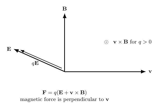
Figure 3. Geometry of the Lorentz force. The electric force points with or against E depending on the sign of q. The magnetic force is perpendicular to both v and B and reverses direction when the charge sign reverses.

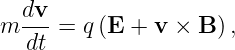
For nonrelativistic particle motion,

dv- m dt = q (E + v × B ),

(33)

with

dr ---= v. dt

(34)

If the fields are known functions of position and time, Equations (33) form an ordinary differential-equation problem for the particle trajectory.

If the moving particle is itself an important source of the fields, the problem becomes self-consistent and much harder.

8 Why magnetic force does no instantaneous work on a point charge

The instantaneous mechanical power delivered by a force is

P = F ⋅ v.

(35)

Using the Lorentz force,

= qE ⋅ v + q(v × B) ⋅ v.

(36)

But

(v × B ) ⋅ v = 0,

(37)

because v × B is perpendicular to v.

Therefore

P = qE ⋅ v.

(38)

The magnetic field can change the direction of a point particle’s velocity, but the magnetic part of the Lorentz force does not directly change that particle’s kinetic energy.

This result will later fit into the much larger energy balance described by Poynting’s theorem.

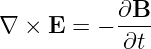
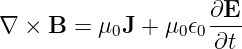
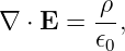
9 A preview of Maxwell’s equations

The ED series will derive, interpret, and apply Maxwell’s Equations gradually. It is useful to see the complete structure now.

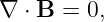
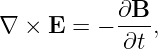
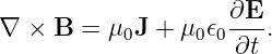
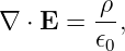
In vacuum with charge density ρ and current density J, the differential equations are

ρ ∇ ⋅ E = --, 𝜖0

(39)

∇ ⋅ B = 0,

(40)

∇ × E = − ∂B--, ∂t

(41)

∂E- ∇ × B = μ0J + μ0 𝜖0∂t .

(42)

Together with the Lorentz force, these equations form the classical core of electrodynamics in vacuum.

At this stage, they should be read structurally rather than memorized as four unrelated formulas.

Charge density appears as a source of electric-field divergence.
The magnetic field has zero divergence, corresponding to the absence of isolated magnetic charge in classical Maxwell theory.
Time-varying magnetic fields are associated with circulating electric fields.
Electric current and time-varying electric fields are associated with circulating magnetic fields.

Later articles will develop every operator and every physical statement in these equations carefully.

10 Constraint equations and evolution equations

The four Maxwell Equations also have an important mathematical structure.

The divergence equations

ρ- ∇ ⋅ E = 𝜖0 ,

(43)

and

∇ ⋅ B = 0

(44)

contain no explicit time derivatives of the fields. They constrain which electric and magnetic field configurations are allowed at a given time.

The curl equations

∇ × E = − ∂B-- ∂t

(45)

and

∂E- ∇ × B = μ0J + μ0𝜖0 ∂t

(46)

contain the time derivatives and therefore participate directly in the evolution of the fields.

These two roles are not independent. Take the divergence of the Ampere-Maxwell equation:

∇⋅ (∇× B)

= μ₀∇⋅ J + μ₀𝜖₀ ∂
---
∂t

(∇⋅ E).

(47)

The divergence of a curl is zero, so

0 = μ0∇ ⋅ J + μ0𝜖0 ∂-(∇ ⋅ E). ∂t

(48)

Using Gauss’s electric law,

∇ ⋅ E = ρ-, 𝜖0

(49)

we obtain

∇ ⋅ J + ∂ρ-= 0. ∂t

(50)

Thus local charge conservation is built into the consistency of Maxwell’s equations.

This also explains why initial fields cannot be specified arbitrarily. Initial data must satisfy the divergence constraints, and the subsequent evolution must remain compatible with the sources.

11 Integral and local laws

Electrodynamics repeatedly uses two descriptions of the same physical law.

An integral law refers to a finite curve, surface, or volume. A local differential law describes what happens in an arbitrarily small neighborhood.

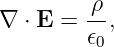
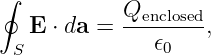
For example, Gauss’s electric law has the integral form

∮ E ⋅ da = Qenclosed, S 𝜖0

(51)

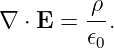
while its local form is

ρ- ∇ ⋅ E = 𝜖0 .

(52)

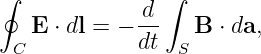
Faraday’s law has the integral form

∮ d ∫ E ⋅ dl = −-- B ⋅ da, C dt S

(53)

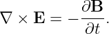
and the local form

∂B ∇ × E = − ----. ∂t

(54)

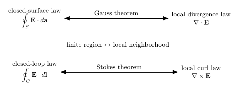
Figure 4. Integral and local viewpoints. Integral laws describe finite curves, surfaces, and volumes. Divergence and curl laws describe the same physics locally. Gauss’s and Stokes’ theorems provide the mathematical bridges between these viewpoints.

ED03 and ED04 will develop the divergence, curl, Gauss theorem, and Stokes theorem carefully enough that these conversions no longer look like formal tricks.

12 Superposition and linearity

Maxwell’s equations in vacuum are linear in the fields and sources.

Suppose source set 1 produces fields

(ρ1,J1) −→ (E1, B1),

(55)

and source set 2 produces

(ρ2,J2) −→ (E2, B2).

(56)

Then the combined sources

ρ = ρ + ρ , J = J + J 1 2 1 2

(57)

produce the combined fields

E = E + E , B = B + B , 1 2 1 2

(58)

provided the medium and constitutive response do not introduce nonlinear behavior.

Superposition is one reason complicated source distributions can be constructed from simpler ones.

It underlies

Coulomb integrals,
Biot-Savart integrals,
multipole expansions,
Green-function solutions,
Fourier and mode expansions,
and many numerical field methods.

Linearity of the field equations does not mean that every electromagnetic problem is easy. Geometry, boundary conditions, moving matter, material response, and self-consistent source motion can all make a linear field equation difficult to solve.

13 Static, quasistatic, and dynamic regimes

Not every electromagnetic problem requires the full time-dependent Maxwell system in its most general form.

The structure of the approximations matters because many practical circuits and laboratory systems are not purely electrostatic or magnetostatic, yet they are also far from the radiation regime.

Electrostatics

Electrostatics assumes source charge distributions do not change with time and the electric field is time independent:

∂ ρ ∂E --- = 0, --- = 0. ∂t ∂t

(59)

The central problems involve charge distributions, electric fields, scalar potential, Conductors, boundary conditions, and electrostatic energy.

Magnetostatics

Magnetostatics assumes steady currents:

∂J ---= 0, ∂t

(60)

with time-independent magnetic fields:

∂B--= 0. ∂t

(61)

The central problems involve current distributions, magnetic fields, vector potential, forces on currents, and magnetic energy.

Quasistatics

A quasistatic system changes with time, but changes slowly enough or over a small enough spatial region that propagation delay and radiation can be neglected to a useful approximation.

If the characteristic size of a system is L and the characteristic timescale is T, define the dimensionless ratio

-L- η = cT .

(62)

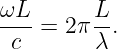
For sinusoidal behavior with angular frequency ω, this is equivalently of order

ωL η ∼ ---. c

(63)

When

η ≪ 1,

(64)

light-crossing time is short compared with the system timescale. Lumped-circuit and quasistatic approximations may then be appropriate.

This criterion does not by itself tell us which quasistatic terms are negligible. Electric quasistatics and magnetic quasistatics emphasize different limits. Later articles will make those approximations more precise.

Fully dynamic electrodynamics

When propagation delay, radiation, retardation, or wave behavior matters, the full time-dependent Maxwell system must be retained.

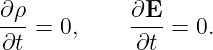
The system can then support electromagnetic waves even where

ρ = 0, J = 0.

(65)

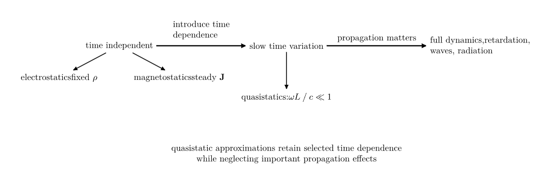
Figure 5. Conceptual regime map. Electrostatic and magnetostatic models occupy time-independent limits. Quasistatic models retain slow time dependence while neglecting important propagation effects. Full electrodynamics is required when retardation, waves, and radiation become significant.

14 A wavelength version of the quasistatic criterion

For harmonic behavior with frequency f,

λ = c. f

(66)

Since

ω = 2πf,

(67)

we have

ωL L --- = 2π --. c λ

(68)

Thus lumped or quasistatic reasoning is most comfortable when

L ≪ λ.

(69)

This is why a centimeter-scale breadboard can often be treated as a lumped circuit at kilohertz frequencies, while the same physical layout may behave very differently at hundreds of megahertz or gigahertz frequencies.

The Radio Build Lab and later EDL transmission-line experiments will make this transition measurable.

15 Boundary data and initial data

Field equations are differential equations. A differential equation alone usually does not specify one unique physical solution.

Static boundary-value problems often require information on the boundaries of the region.

For example, solving Laplace’s equation

∇2V = 0

(70)

requires appropriate boundary data such as the potential on conducting surfaces.

Time-dependent electromagnetic problems also require initial data consistent with Maxwell’s constraints.

Schematically,

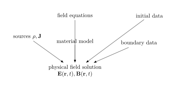
field equations + sources + boundary data + initial data −→ physical solution.

(71)

Figure 6. Field equations are not enough by themselves. Sources, material properties, boundary conditions, initial conditions, and sometimes radiation conditions are all part of specifying a unique electromagnetic problem.

This perspective will become central in electrostatic uniqueness theorems, Green functions, waveguides, cavities, and radiation problems.

16 Locality and causal propagation

Static formulas can make Electromagnetism look instantaneous.

For example, Coulomb’s electrostatic field of a point charge has the familiar form

1 E ∝ --ˆr. r2

(72)

If the source moves, however, the field at a distant point does not update everywhere instantaneously.

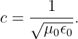
Changes propagate through the electromagnetic field at the finite speed

c = ---1--. √ μ0𝜖0

(73)

The full theory therefore has a local dynamical structure:

sources affect fields in their neighborhood according to Maxwell’s equations;
field disturbances propagate through space;
fields locally exert force on charged matter;
electromagnetic energy and momentum can reside in and move through the field.

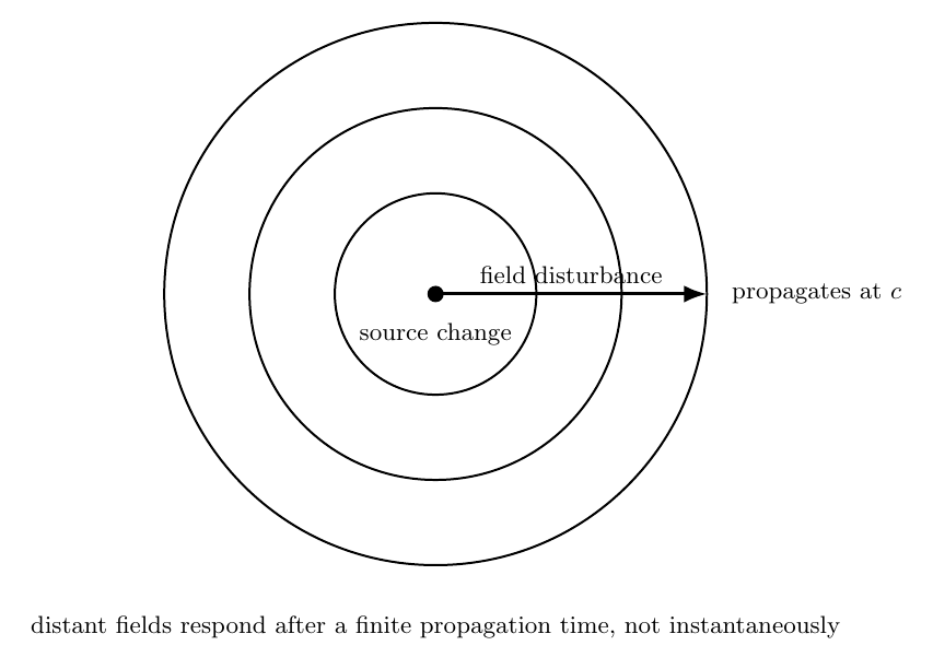
Figure 7. Static field formulas are limiting solutions, not evidence for instantaneous physical influence. In the dynamical theory, changes in source motion alter the electromagnetic field and the disturbance propagates outward at finite speed.

The retarded-potential and radiation articles later in the ED series will make this causal structure explicit.

17 Fields are dynamical degrees of freedom

The field viewpoint becomes especially clear in a region containing no charge and no current.

Suppose

ρ = 0, J = 0.

(74)

Maxwell’s equations do not then require

E = 0, B = 0.

(75)

Instead, time-varying electric and magnetic fields can sustain one another and propagate as waves.

This is a major conceptual step beyond static action-at-a-distance thinking. The electromagnetic field has its own dynamical behavior.

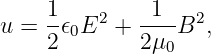
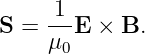
Later we will associate the fields with energy density

1 1 u = -𝜖0E2 + ---B2, 2 2μ0

(76)

and energy flux described by the Poynting vector

S = -1-E × B. μ0

(77)

These are previews. ED47 develops the energy balance in detail.

18 SI units and dimensional checks

Dimensional analysis is one of the fastest ways to catch an electrodynamics mistake.

Some central SI units are

Quantity	Symbol	SI unit

charge	q	C
charge density	ρ	C/m³
current	I	A
current density	J	A/m²
electric field	E	N/C = V/m
magnetic field	B	T
electric potential	V	V = J/C
permittivity of vacuum	𝜖₀	F/m
permeability of vacuum	μ₀	H/m

As an example, the electric part of the Lorentz force is

FE = qE.

(78)

Its units are

( ) N- C C = N.

(79)

For the magnetic part,

FB = qv × B,

(80)

so Tesla must be consistent with

-N-- T = A m .

(81)

Then

[qvB]	= C	(82)
	= N,	(83)

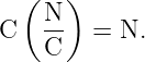
because

A = C∕s.

(84)

Every major derivation in the ED series should include this kind of unit check when it is useful.

19 A simple source-field-response example

Consider a fixed point charge Q at the origin. ED09 will derive the electrostatic field from Coulomb’s law. Here we use the result only to illustrate the structure of the theory.

The source is

Q.

(85)

At a field point r a distance

r = |r|

(86)

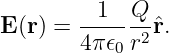
from the charge, the electric field is

E (r) = --1--Q-ˆr. 4π 𝜖0r2

(87)

Now place a small test charge q at that point. If the test charge is momentarily at rest, its force is

F	= qE	(88)
	= r.	(89)

The calculation naturally separates into two stages:

Q − → E(r) −→ F (q).

(90)

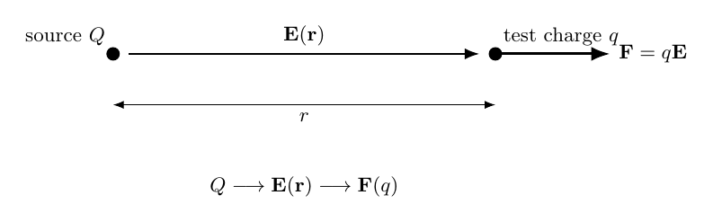
Figure 9. Source-field-response decomposition for the electrostatic interaction of two charges. The source charge Q establishes a field at the test location. The test charge q responds to the local field through F = qE.

This separation becomes much more valuable for complicated source distributions because the field exists as a function over space, independent of which particular test charge is later used to probe it.

Numerical example

Let

Q = 2.0 nC, r = 0.10 m.

(91)

Using

--1-- 9 2 2 4π 𝜖0 ≈ 8.99 × 10 N m ∕C ,

(92)

the field magnitude is

E	=	(93)
	≈ (8.99 × 10⁹)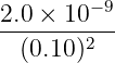	(94)
	≈ 1.80 × 10³ N∕C.	(95)

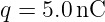
If a test charge

q = 5.0 nC

(96)

is placed there, then

F	= qE	(97)
	≈ (5.0 × 10⁻⁹)(1.80 × 10³)	(98)
	≈ 9.0 × 10⁻⁶ N.	(99)

The source-field-response structure has separated the problem into an environmental property, E, and the response of a particular probe, q.

20 What does a laboratory instrument actually measure?

The phrase “measure the electric field” can hide several layers of physical inference.

A voltmeter does not directly display the vector field E. It measures a potential difference between two terminals by allowing a small current to flow through its input circuit and then inferring voltage from the instrument response.

An oscilloscope displays voltage as a function of time relative to a reference terminal. Its input resistance and capacitance load the circuit being measured.

A current measurement may be inferred from the voltage across a known resistor:

I = VR-. R

(100)

A Hall probe infers magnetic field from a material response that has been calibrated against B.

A field-mapping experiment may measure many values of electric potential and reconstruct the electric field from

E = − ∇V.

(101)

Thus most instruments measure an observable that is connected to the desired field through a model.

Figure 8. Measurement is an inference chain. A physical field interacts with a probe, the probe produces an electrical or mechanical response, an instrument converts that response into data, and a model is used to infer the desired physical quantity.

This is why EDL01 spends so much time measuring the measuring system itself.

21 Connection to EDL01

EDL01 introduces practical electricity and measurement before the laboratory series attempts to map fields.

That lab measures quantities such as

DMM input resistance,
function-generator source resistance,
oscilloscope probe loading,
common oscilloscope grounding,
resistor tolerance,
and RC time constants.

Those are not separate from electrodynamics. They determine how the ideal variables in our field and circuit models are connected to actual measurements.

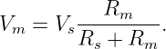
For example, suppose an ideal source would produce voltage V _s, but the source has finite resistance R_s and the measuring instrument has input resistance R_m.

The measured voltage is

Vm = Vs---Rm----. Rs + Rm

(102)

Only when

R ≫ R m s

(103)

do we have

Vm ≈ Vs.

(104)

The measurement apparatus has become part of the physical system.

That lesson will recur in every EDL article.

22 Fields, potentials, and redundancy

The electromagnetic fields E and B can be represented in terms of potentials.

Later we will define a scalar potential V and vector potential A such that

B = ∇ × A,

(105)

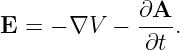
and, in the general time-dependent case,

∂A E = − ∇V − ----. ∂t

(106)

The potentials contain a redundancy called gauge freedom. Different potentials can represent the same physical fields.

This will initially appear to be a mathematical convenience. By the time we reach retarded potentials and relativistic notation, the potentials will become central computational objects.

ED42 through ED46 develop this structure carefully.

23 Matter introduces additional modeling

The vacuum Maxwell equations use ρ and J as sources.

Macroscopic matter introduces additional concepts such as

P, M, D, H,

(107)

representing polarization, magnetization, and auxiliary fields useful for separating free and bound sources.

These quantities are not new Fundamental interactions added to Maxwell’s theory. They are macroscopic ways of organizing the electromagnetic response of matter.

The constitutive behavior of matter may be

linear or nonlinear,
isotropic or anisotropic,
local or spatially dispersive,
instantaneous or frequency dependent,
lossless or dissipative.

Thus the simple statement

D = 𝜖E

(108)

is a model with a domain of validity, not a universal definition of all dielectric matter.

ED23 through ED28 and ED34 through ED36 develop these material models.

24 The classical domain of the theory

Classical electrodynamics is enormously successful, but it is not the final description of nature at all scales.

The classical theory is generally appropriate when the relevant electromagnetic fields and charged matter can be treated without requiring a quantum description of individual emission, absorption, atomic structure, or particle creation.

At very high velocities, the particle mechanics must be relativistic. Maxwell’s field theory itself is already compatible with special relativity, and ED66 through ED72 make that connection explicit.

At microscopic quantum scales, classical fields and classical particle trajectories may no longer provide a complete description.

The ED series remains a classical theory series. Its purpose is to understand that theory deeply enough that the boundaries of the classical description are also clear.

25 A useful problem-solving hierarchy

When approaching an electrodynamics problem, first identify the level of description.

Identify the sources: point charges, ρ, J, polarization, magnetization, or prescribed boundary data.
Decide whether the problem is static, quasistatic, or fully dynamic.
Identify the desired field or potential.
Write the governing Maxwell or potential equation appropriate to that regime.
Identify symmetry, boundary conditions, and initial conditions.
Solve for the field.
Convert the field into the desired observable: force, energy, voltage, flux, power, momentum, or detector response.
Check units, limits, symmetry, and conservation laws.
Ask what an experiment would actually measure.

This hierarchy is more reliable than searching immediately for a memorized formula.

26 Companion files

Two compact reference files accompany this article in the PhysicsLibrary filebox.

These files are intended as quick references while working later ED and EDL articles.

27 Summary

The basic architecture of classical electrodynamics is

(ρ,J) −→ (E,B ) −→ F = q(E + v × B ).

(109)

Charge conservation connects the source variables through

∂ρ-+ ∇ ⋅ J = 0. ∂t

(110)

Maxwell’s equations determine how the fields are related to sources and to one another.

Superposition allows complicated source distributions to be assembled from simpler ones.

Static and quasistatic approximations are limiting regimes of the full dynamical theory, not separate laws of nature.

Boundary and initial data are part of specifying a field problem.

Fields are dynamical physical quantities that can carry energy and momentum and propagate through vacuum.

Laboratory instruments generally infer fields through calibrated physical responses; they do not passively reveal an ideal mathematical variable without interacting with the system.

The next article, ED02, develops the vector and coordinate geometry required to describe fields precisely.

References

[1] D. J. Griffiths, Introduction to Electrodynamics, 5th ed., Cambridge University Press, 2023.

[2] E. M. Purcell and D. J. Morin, Electricity and Magnetism, 3rd ed., Cambridge University Press, 2013.

[3] A. Zangwill, Modern Electrodynamics, Cambridge University Press, 2013.

[4] R. P. Feynman, R. B. Leighton, and M. Sands, The Feynman Lectures on Physics, Volume II, Addison-Wesley.

[5] J. D. Jackson, Classical Electrodynamics, 3rd ed., Wiley, 1999.

"The Physical Structure of Classical Electrodynamics" is owned by bloftin.
(view preamble)

The Physical Structure of Classical Electrodynamics

ED01: The Physical Structure of Classical Electrodynamics

1 The physical objects of the theory

2 Point sources and continuous sources

3 Current density

4 Charge conservation

5 What is an electromagnetic field?

6 The operational idea of a test charge

7 The Lorentz force

8 Why magnetic force does no instantaneous work on a point charge

9 A preview of Maxwell’s equations

10 Constraint equations and evolution equations

11 Integral and local laws

12 Superposition and linearity

13 Static, quasistatic, and dynamic regimes

Electrostatics

Magnetostatics

Quasistatics

Fully dynamic electrodynamics

14 A wavelength version of the quasistatic criterion

15 Boundary data and initial data

16 Locality and causal propagation

17 Fields are dynamical degrees of freedom

18 SI units and dimensional checks

19 A simple source-field-response example

Numerical example

20 What does a laboratory instrument actually measure?

21 Connection to EDL01

22 Fields, potentials, and redundancy

23 Matter introduces additional modeling

24 The classical domain of the theory

25 A useful problem-solving hierarchy

26 Companion files

27 Summary

References

References

Pending Errata and Addenda

Discussion

Interact