|
|
|
|||||||
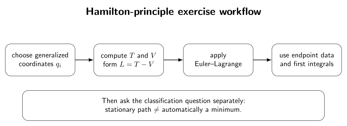
The central message was that the physical trajectory is a stationary trajectory of the action, not automatically a minimizing trajectory. This exercise set develops that statement computationally. The problems begin with the free particle and uniform gravity, then move through the harmonic oscillator, pendulum, generalized coordinates, cyclic coordinates, conserved energy, total-derivative changes of the Lagrangian, and natural endpoint conditions. These are standard themes in analytical mechanics [1, 2, 3, 4] and they connect directly to the variational machinery developed earlier in this series [5].
Figure. A practical workflow for Hamilton-principle exercises. The coordinates and energy model define L; the Euler–Lagrange equations determine stationary trajectories; symmetries supply first integrals; and CV11–CV13 determine whether a stationary path is actually minimizing.
1 Exercises
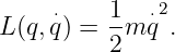
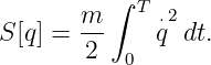
Exercise 1: free particle with fixed endpointsA particle of mass m moves in one dimension with
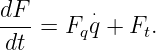
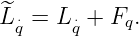
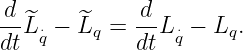
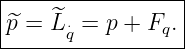
The endpoint conditions are
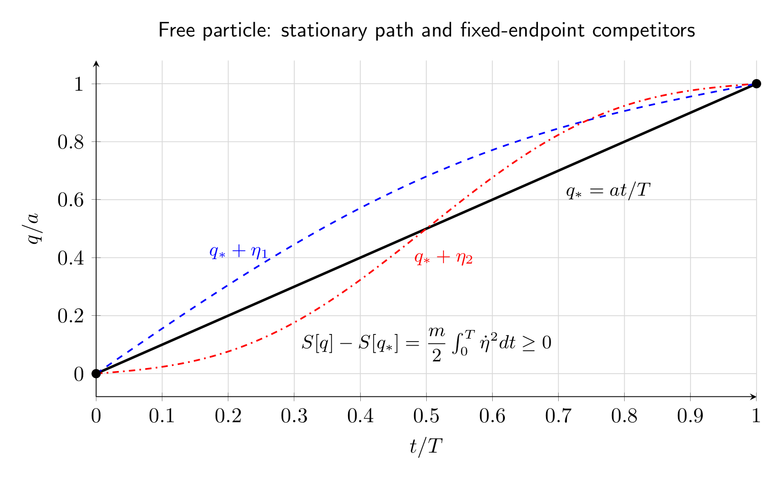
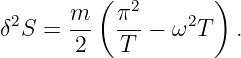
Figure. The straight worldline in the (t,q) plane is stationary. For the free-particle
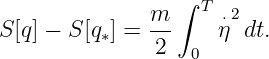
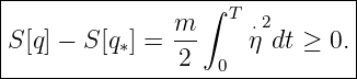
quadratic action, every nonzero fixed-endpoint perturbation adds the positive amount
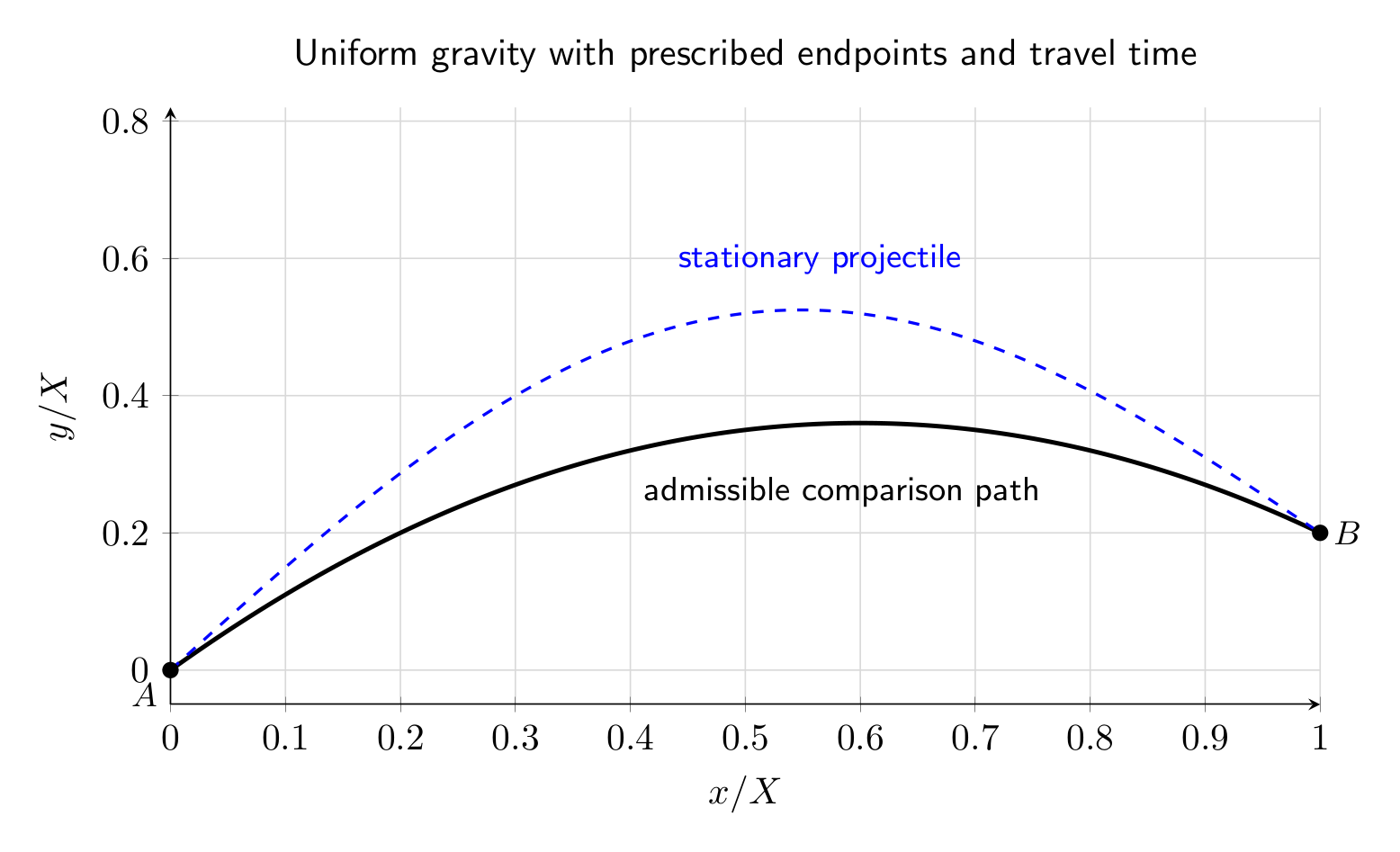
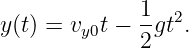
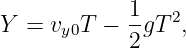
Exercise 2: a projectile between prescribed spacetime endpointsA particle moves in the vertical plane under uniform gravity. Use
The particle must travel from
to
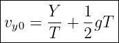
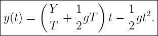
Figure. Uniform gravity with fixed spacetime endpoints. The endpoint conditions determine the initial velocity required for the stationary projectile trajectory.
Exercise 3: harmonic oscillator boundary-value problem and critical timeFor
impose
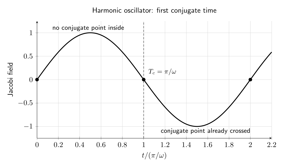
Figure. The first harmonic-oscillator conjugate time is π∕ω. The same stationary equation persists on longer intervals, but the minimizing character changes.
Exercise 4: the simple pendulumA pendulum of mass m and length ℓ is described by the angle 𝜃 from the downward vertical.
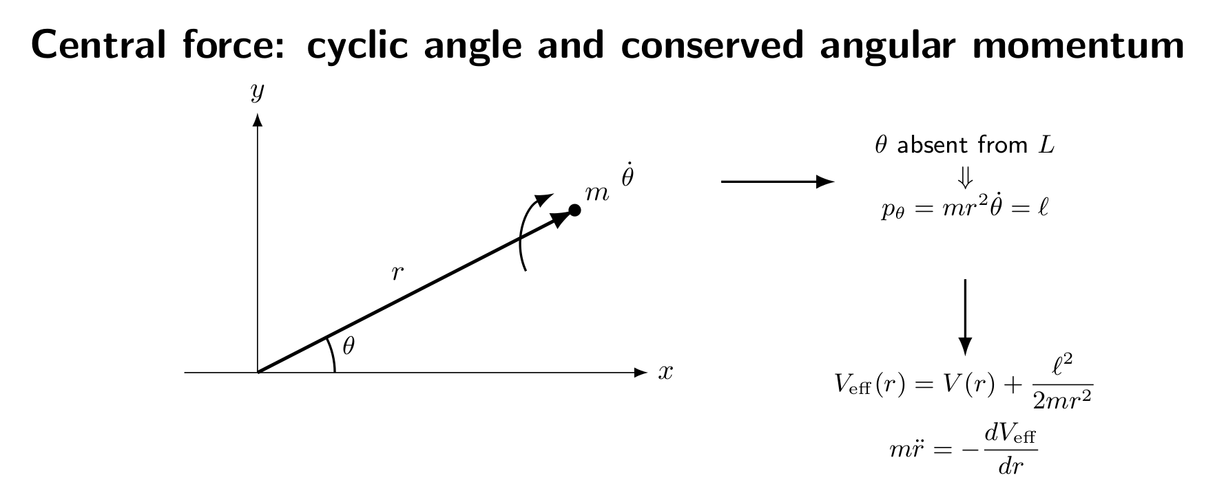
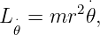
Exercise 5: a central force and a cyclic angleFor planar motion in polar coordinates, take
Figure. Rotational symmetry makes 𝜃 cyclic. Conservation of p𝜃 = mr2
Exercise 6: deriving the energy identity for an arbitrary LagrangianLet
and define
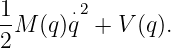
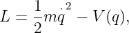
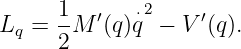
Exercise 7: a generalized coordinate with coordinate-dependent inertiaConsider
Exercise 8: adding a total time derivative to the LagrangianLet
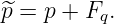
Exercise 9: free terminal position and the momentum boundary termConsider
with fixed initial position q(t1), fixed endpoint times, but free terminal position q(t2).
2 Worked solutions
Solution 1: free particle with fixed endpointsThe action is
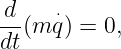
The Euler–Lagrange equation is
so
Hence
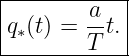
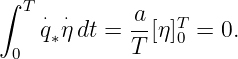
The boundary conditions give B = 0 and AT = a, so
The stationary action is
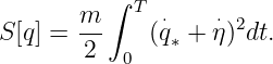
Now write
Then
Expanding the square gives
Because
Therefore
Equality requires
Solution 2: a projectile between prescribed spacetime endpointsFor x,
so
For y,
so
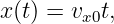
Integrating,
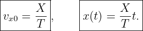
because x(0) = 0. Since x(T) = X,
Similarly,
The terminal condition gives
hence
and
When X≠0,
so
which is a parabola. The varied paths used in the action comparison are not required to obey
Solution 3: harmonic oscillator boundary-value problem and critical timeThe Euler–Lagrange equation is
or
The general solution is
Since q(0) = 0, B = 0. Therefore
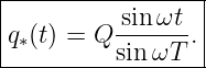
If sin ωT≠0,
If Q≠0 and sin ωT = 0, the equation Q = A sin ωT cannot be satisfied. There is no classical stationary trajectory with those fixed endpoint data and that prescribed travel time. If Q = 0 and
then
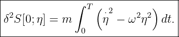
satisfies both endpoints for every real A. The boundary-value problem is therefore degenerate. Along q∗ = 0, the action is quadratic, so the second variation is
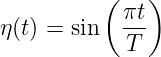
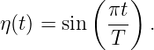
Take
Using
we obtain
The first sign change occurs at
Thus:
This is exactly the CV11–CV12 distinction between stationarity and conjugate-point loss of minimizing character.
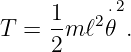
Solution 4: the simple pendulumThe bob speed is
so
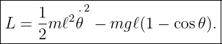
With the downward vertical as zero potential,
Hence
Now
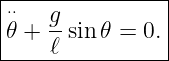
Therefore
or
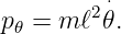
The generalized momentum is
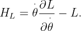
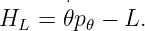
Because L has no explicit time dependence,
Substituting the pendulum Lagrangian,
so
For small angles,
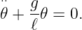
and the equation becomes
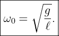
Therefore
Hamilton’s principle produced the exact nonlinear equation. The approximation enters only afterward when sin 𝜃 is replaced by 𝜃.
Solution 5: a central force and a cyclic angleSince L contains 𝜃 only through
Therefore
But
so
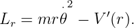
For r,
and
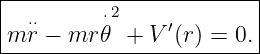
Hence
Using
we obtain
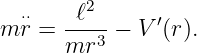
Define
Then
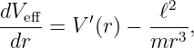
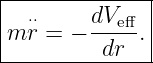
and the radial equation becomes
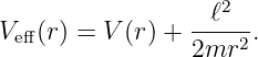
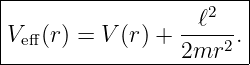
For ℓ≠0, the effective term
diverges as r → 0. It therefore produces an angular-momentum barrier against reaching the origin unless the original potential is sufficiently singular to overcome it.
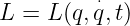
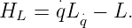
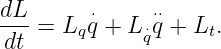
Solution 6: deriving the energy identity for an arbitrary LagrangianStart from
Differentiate:
The total derivative of L is
Substitution gives
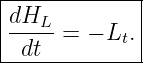
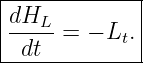
Along an Euler–Lagrange trajectory, the parenthesis vanishes. Therefore
If Lt = 0,
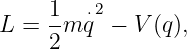
For
we have
so
Thus ordinary mechanical energy appears as a first integral of the Euler–Lagrange equation when the Lagrangian is autonomous.
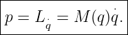
Solution 7: a generalized coordinate with coordinate-dependent inertiaThe generalized momentum is
Next,
Also,
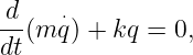
The Euler–Lagrange equation therefore gives
hence
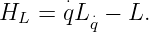
The energy function is
Because M and V can depend on q, the coordinate q is not generally cyclic. Therefore p = M
that is, if q were cyclic.
Solution 8: adding a total time derivative to the LagrangianBy the chain rule,
Therefore
Compute
Then
Also,
Since mixed partial derivatives agree,
we get
Thus L and L produce exactly the same Euler–Lagrange equation. At the action level,
For fixed endpoint data this is a fixed number, so the two actions have the same stationary paths. However,
Thus a total derivative leaves the motion unchanged while shifting the canonical momentum. This is one reason canonical quantities must be interpreted with care.
Solution 9: free terminal position and the momentum boundary termLet
with
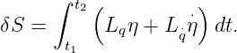
but no restriction on η(t2). The first variation is
Integrate by parts:
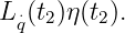
The initial boundary contribution vanishes because η(t1) = 0. Stationarity for arbitrary interior variations gives the Euler–Lagrange equation. The remaining terminal term is
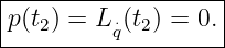
Because the terminal position is free, η(t2) is arbitrary. Hence
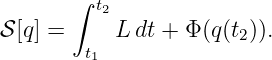
Now consider
The endpoint cost varies as
Therefore the total terminal contribution is
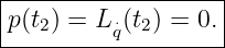
Stationarity for arbitrary η(t2) gives
This is the mechanics form of the natural boundary-condition logic developed in CV05: generalized momentum is literally the coefficient multiplying the free endpoint displacement in the first variation.
3 What these exercises add to CV14The examples above expose several structural facts that are easy to miss if Hamilton’s principle is treated only as a formal recipe.
These points are standard in analytical mechanics treatments [1, 2, 4]. They also prepare the next main lesson, CV15, where constraints and generalized coordinates are developed systematically.
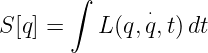
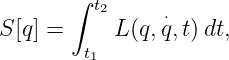
SummaryHamilton’s principle starts with
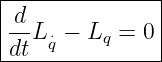
and demands stationarity under admissible path variations. The resulting Euler–Lagrange equation
contains Newtonian dynamics, but its variational origin also reveals more structure: generalized momentum, cyclic-coordinate conservation, energy conservation, natural endpoint conditions, and the distinction between stationary and minimizing trajectories. The exercises show that the same framework handles straight-line free motion, projectile trajectories, oscillations, pendulum dynamics, central forces, coordinate-dependent kinetic energy, equivalent Lagrangians, and terminal boundary conditions. The calculations therefore provide a practical bridge from the formal calculus of variations to classical analytical mechanics.
References
[1] Cornelius Lanczos, The Variational Principles of Mechanics, 4th ed., Dover Publications, 1986. [2] Herbert Goldstein, Charles Poole, and John Safko, Classical Mechanics, 3rd ed., Addison-Wesley, 2002. [3] L. D. Landau and E. M. Lifshitz, Mechanics, 3rd ed., Butterworth-Heinemann, 1976. [4] V. I. Arnold, Mathematical Methods of Classical Mechanics, 2nd ed., Springer, 1989. [5] I. M. Gelfand and S. V. Fomin, Calculus of Variations, Dover Publications, 2000. "Calculus of Variations: Hamilton's Principle and Classical Mechanics - Exercises" is owned by bloftin.
This object's parent. Cross-references: central forces, identity, formula, displacement, mechanical energy, nonlinear equation, speed, force, square, boundary, CV05, position, energy conservation, radial equation, effective potential, angular momentum, momentum, polar coordinates, frequency, function, potential energy, kinetic energy, second variation, spacetime, velocity, dimension, mass, mechanics, Lagrangian, energy, generalized coordinates, oscillator, particle, Hamilton's principle, CV14 This is version 1 of Calculus of Variations: Hamilton's Principle and Classical Mechanics - Exercises, born on 2026-10-20. Object id is 1510, canonical name is CalculusOfVariationsHamiltonsPrincipleAndClassicalMechanicsExercises. Accessed 5 times total. Classification:
|
|
|
|
Pending Errata and AddendaNone.
|
DiscussionNo messages.
|
Interact |













 in favor of the constant
 reduces the
two-coordinate problem to one


 is generally not conserved even though energy is conserved.










 = 0, so






 = 0 and
 =















 ,















 is
not generally conserved. It would be conserved only if