
|
|
|
|||||||
Every formula will be checked in familiar coordinates, including a nonorthogonal chart in which off-diagonal metric coefficients cannot be ignored.
1 Preliminary distinction: geometry versus coordinatesWe begin in ordinary three-dimensional Euclidean space. A point has a position vector r, and the physical squared length of a small displacement is
This statement does not depend on whether the point is labeled by Cartesian, cylindrical, spherical, or some unusual curvilinear coordinates. What changes is the expression for dr in terms of the chosen coordinate differentials. One should distinguish three things:
The metric tensor records how coordinate increments combine into the physical length in Equation (1).
2 Understanding upper and lower indices before deriving the metricWe use coordinates q1,q2,q3. The superscript here is an index label, not an exponent. In particular, q2 names the second coordinate; it does not mean (q1)2. Thus the position map is
We use indices i,j,k,… taking the values 1, 2, 3. A repeated index, once in an upper position and once in a lower position, means summation over these three values. This is Einstein summation convention. For example,
where i is a dummy index. It can be renamed consistently without changing the sum:
By contrast, k is a free index in
There are three equations, one for each value of k:
The number of free indices must agree on both sides of an equation. A dummy index must be summed exactly once; in conventional index notation it appears once up and once down. Repeated letters must not accidentally be used for two different sums. An ordinary partial derivative is abbreviated
Here ∂i carries a lower index because the partial derivatives of a scalar transform as components of a covector. We will derive the relevant transformation law instead of simply asserting it.
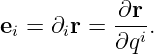
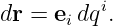
3 The coordinate basis comes from differentiating the position mapApply the multivariable differential rule to Equation (2):
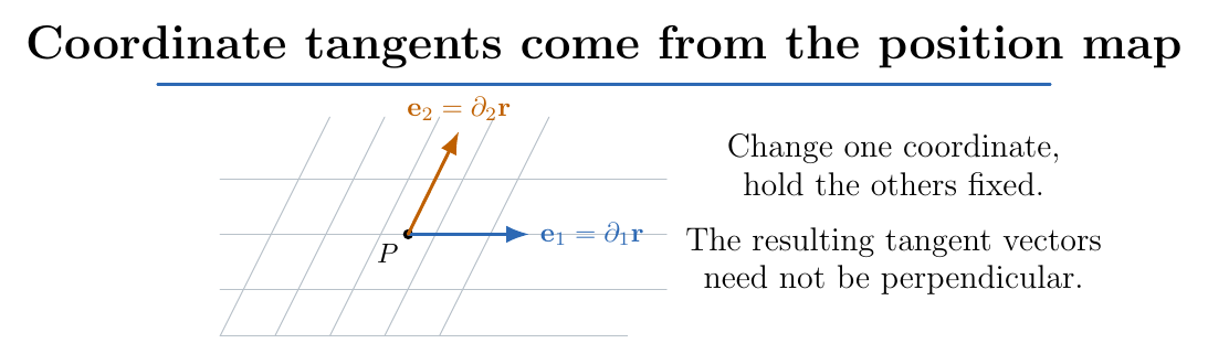
Define three tangent vectors
They are called the coordinate basis or covariant basis vectors. They are not necessarily unit vectors and are not necessarily perpendicular. With this definition, Equation (7) becomes
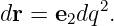
Explicitly, this says dr = e1dq1 + e 2dq2 + e 3dq3. If only coordinate q2 changes, the local displacement is
Thus e2 is the tangent to the curve obtained by varying q2 while keeping the other coordinates fixed.
Figure 1. Local coordinate tangents arise by varying one coordinate at a time. Their lengths and mutual angles, rather than just their names, determine the metric.
4 The metric tensor emerges from the squared lengthReturn to physical squared length:
Substitute Equation (9):
The scalar coordinate differentials can be taken outside the dot product:
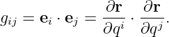
The coefficients are so important that we name them:
We have thus derived the line-element relation
No advanced geometry was assumed. The metric coefficients are the dot products of the coordinate tangent vectors.
What the indices actually sayFor three coordinates, Equation (15) expands to
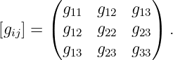
Why the factors of two? Because g12 = g21, and the full double sum contains both g12dq1dq2 and g21dq2dq1. The metric matrix is
It is symmetric because dot products commute:
For any nonzero coordinate increment, in a nonsingular Euclidean chart,
Thus the metric is positive definite wherever the coordinates are regular.
5 Lengths and angles are hidden inside the metric matrixSet dq2 = dq3 = 0. Then
Therefore the physical distance along the first coordinate line is
This recovers the familiar scale factor
But the metric gives more information. The angle α12 between the first two coordinate tangent vectors satisfies
Thus the diagonal terms measure squared tangent lengths, while the off-diagonal terms measure the failure of coordinate directions to be orthogonal. For orthogonal coordinates, gij = 0 when i≠j and
The ED02/ED06 formula
is therefore the orthogonal special case, not the definition of the metric.
6 Why the metric is a tensor: a coordinate-change proofConsider two coordinate descriptions of the same region:
Apply the chain rule to the position vector:
The metric in the new chart is
This is exactly the transformation rule for a covariant rank-two tensor. It guarantees that the squared physical length is unchanged by relabeling points:
In matrix notation, if Ji a = ∂qi∕∂qa, then
The entries change, but the physical length does not. This is why we call gij a tensor, rather than merely a table of coordinate-dependent coefficients.
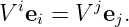
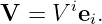
7 Contravariant and covariant vector componentsA physical vector V can be expanded in the coordinate basis:
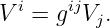
The coefficients V i are its contravariant components. This is consistent with the differential displacement dr = dqie i, for which the components are dqi. Define the covariant components by taking dot products:
Substitute Equation (35):
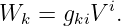
This is called lowering an index with the metric. It is simply the operation of converting vector coefficients into dot products with the coordinate basis.
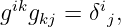
The inverse metricLet [gij] be the matrix inverse of [g ij]:
where the Kronecker delta δi j equals one if i = j and zero otherwise. Multiplying Equation (39) by gki gives
Thus
The inverse metric gij is not generally obtained by taking the reciprocal of each metric entry. One must invert the full matrix. Element-by-element reciprocals work for the diagonal entries only in a diagonal metric.
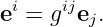
Reciprocal basisDefine the reciprocal vector basis by
Then
Consequently
with
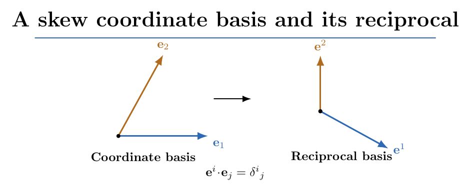
The coordinate basis and the reciprocal basis need not be parallel in a nonorthogonal chart. This is why upper and lower indices are useful rather than decorative.
Figure 2. In a skew coordinate chart, the two tangent basis vectors are not perpendicular, and the reciprocal basis is different. The reciprocal vectors isolate the corresponding contravariant components by dot product.
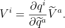
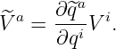
8 Why vector and covector components transform differentlyThe metric transformation law is useful, but the notation becomes much more intuitive if we also derive the transformations of vector components and scalar derivatives. Start with the same physical vector expressed in two coordinate bases:
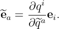
Use the transformation of coordinate basis vectors,
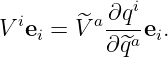
Then
The basis vectors are linearly independent, so their coefficients agree:
Multiply by the Jacobian of the inverse coordinate transformation:
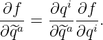
The coordinate basis vectors and their contravariant components transform oppositely so that the physical vector remains unchanged. Next consider a scalar f. The chain rule gives
These derivatives transform with the same Jacobian as the lower-index metric, not the inverse Jacobian of Equation (53). They are the components of a covector or one-form df. The metric is exactly what converts between the two types of components:
These are not merely notation rules. Raising the index on ∂if is the operation that will turn the scalar field’s derivatives into the physical gradient vector.
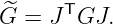
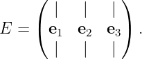
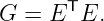
9 The metric as a Gram matrixFor a small physical displacement, write the columns of a 3 × 3 matrix as the three coordinate tangent vectors:
Here each vector column is understood through its Cartesian components. Then
The matrix G is a Gram matrix: it contains every pairwise dot product of the basis vectors. Its determinant measures the squared volume spanned by them. Indeed,
Thus, for a nondegenerate chart,
This is the algebraic bridge between the metric and the familiar Jacobian determinant of multivariable calculus.
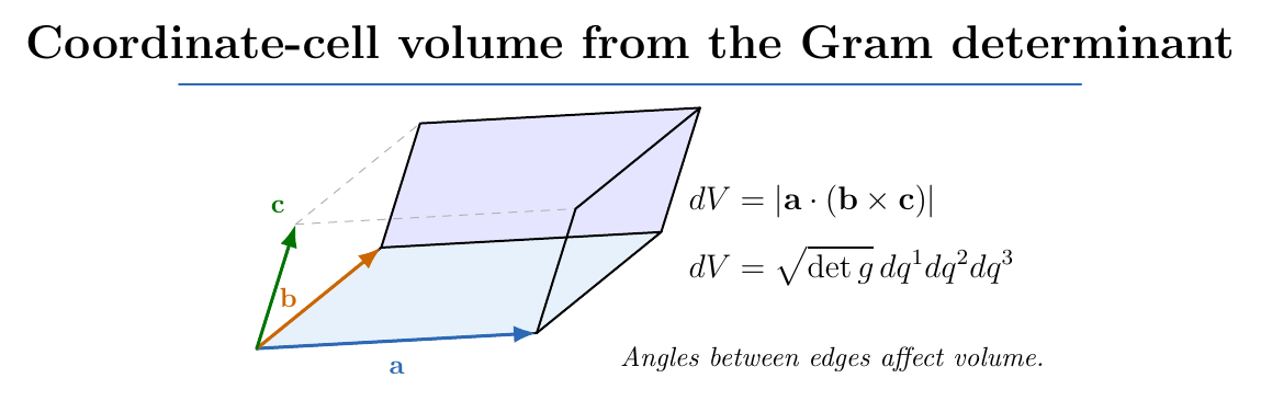
10 Derivation of the volume element from the metricA small coordinate cube has edge displacement vectors
Its unsigned physical volume is the magnitude of the scalar triple product:
Substitute the three edges:
Use Equation (61):
For increasing, positively oriented coordinate intervals, we commonly write
Notice that g in this expression denotes the determinant of the metric matrix, not a gravitational acceleration.
Figure 3. Three small coordinate changes generate a skew parallelepiped. Its volume is a scalar triple product; the same number is obtained from the square root of the metric determinant.
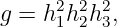
Connection to ED06 scale factorsFor orthogonal coordinates,
Then
so
This reproduces ED06. The determinant formula is its generalization to nonorthogonal coordinate systems.
11 Derivation of a surface metric and its area elementA surface need not be defined by a constant coordinate in an existing three-dimensional chart. It may be given independently by two parameters (u,v):
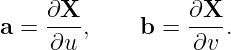
Its tangent vectors are
An infinitesimal displacement within the surface is
Take the squared length:
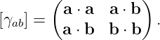
Define the induced surface metric
Thus
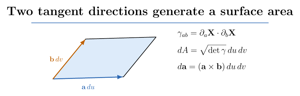
The physical infinitesimal parallelogram has edges adu and bdv, so
Use Lagrange’s identity
The right-hand side is precisely
Therefore
An oriented area vector also retains the surface Normal:
Equation (81) gives its magnitude. Equation (82) gives the corresponding orientation for an ordered surface parameterization.
Figure 4. Two surface parameters generate tangent vectors a and b. The induced metric gives their lengths and angle, while the cross product gives the oriented surface area.
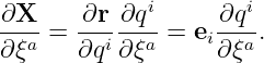
Surface metric from an ambient coordinate metricSuppose the surface is described in a three-dimensional curvilinear chart by qi = qi(ξ1,ξ2). The physical tangent to the first surface coordinate is
The induced metric is its tangent-vector dot product:
Thus the surface metric is obtained by restricting the ambient metric to the directions tangent to the surface. This construction works even if the surface is not a coordinate surface of the ambient chart.
A subtle distinctionThe full three-dimensional determinant det g controls three-dimensional volume; the induced
two-dimensional determinant det γ controls two-dimensional area. One should not insert
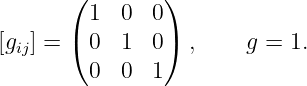
12 Example: Cartesian metricThe Cartesian position map is
Its coordinate tangents are
Consequently
The line and volume elements are the familiar
13 Example: cylindrical metric from the position mapUse (q1,q2,q3) = (s,ϕ,z) with
Differentiate one coordinate at a time:
The dot products give
Therefore
The line element is
Its determinant and square root are
Thus
We recover all the ED02/ED06 scale factors from the metric without memorizing a separate volume rule.
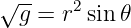
14 Example: spherical metric and the surface patchChoose (q1,q2,q3) = (r,𝜃,ϕ) with 𝜃 measured down from +z:
Differentiate with respect to r:
Differentiate with respect to 𝜃:
Differentiate with respect to ϕ:
The tangent magnitudes are
for r > 0 and 0 < 𝜃 < π. All off-diagonal dot products vanish. Hence
The physical line element is
The determinant is
which gives
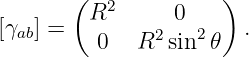
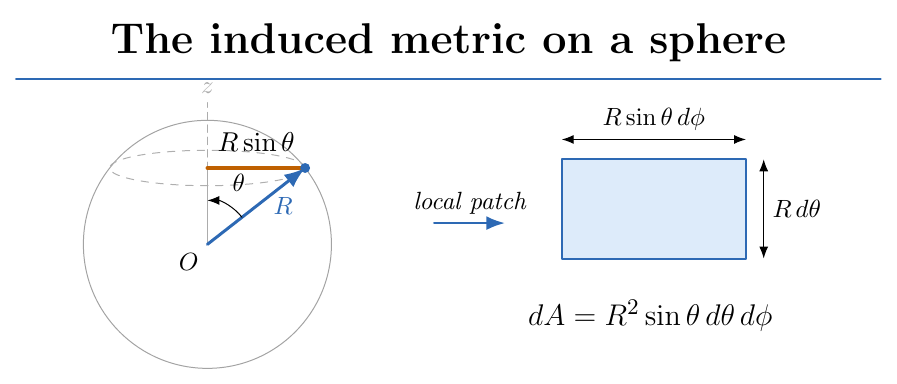
Induced metric of a sphereNow hold r = R constant. The surface parameters are (𝜃,ϕ), so the surface metric is obtained from ∂𝜃r and ∂ϕr:
Its determinant is
Therefore
The origin of the sine is now explicit: a change dϕ at fixed polar angle runs along a parallel circle of radius R sin 𝜃, so its physical length is R sin 𝜃 dϕ.
Figure 5. The sphere’s meridian and parallel directions have physical scale factors R and R sin𝜃. Multiplying their differential lengths gives the induced-metric surface area.
15 An essential example: nonorthogonal coordinatesThe real strength of the metric tensor becomes clear when the coordinate axes are skew. Start with Cartesian (x,y,z) and define new coordinates (u,v,w) by
where k is a fixed dimensionless shear parameter. The position vector is
Its coordinate tangents are
Take their dot products one by one:
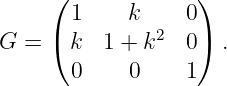
The metric is
Its off-diagonal terms produce a cross term in the line element:
The determinant is
Hence
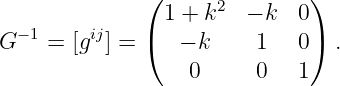
This is an instructive result. The coordinate cell is tilted, but this shear preserves volume. Multiplying the three individual edge lengths would give the wrong volume because the edges are not mutually perpendicular. The determinant takes their angles into account. The inverse metric is
This example will also test the Laplace–Beltrami formula below.
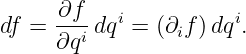
16 From the metric to a gradientLet f be a scalar field. Its ordinary total differential is
The physical gradient is defined by the condition
for every infinitesimal physical displacement. Expand the unknown gradient in the coordinate basis:
Substitute dr = eidqi into Equation (119):
Compare with Equation (118). Since the dqi are independent,
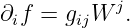
Multiply by the inverse metric:
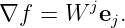
Therefore
The coordinate components of the gradient vector are
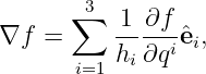
This derivation explains why the inverse metric appears: the derivatives ∂if are covariant components, and converting them to vector components requires raising an index. For orthogonal coordinates, gii = 1∕h i2 and e i = hiei, giving
exactly as in ED03 and ED06.
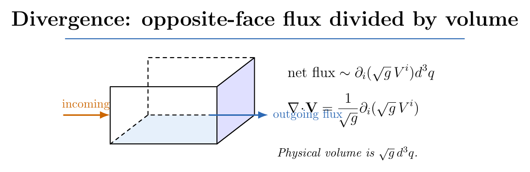
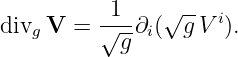
17 Divergence from the physical volume measureFor a vector field V = V ie i, divergence measures local outward flux per unit physical volume. In a general coordinate chart, the physical volume element is
Consider a small coordinate cell. On the faces q1 = constant, the oriented area vector per coordinate area is
A useful algebraic identity for a right-handed regular chart is
where 𝜖ijk is the alternating symbol with 𝜖123 = 1. The positive flux through the q1 face is consequently
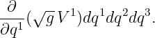
The fluxes through the two opposing q1 faces differ to first order by
Adding the analogous q2 and q3 pairs gives total outward flux
Divide by the physical volume
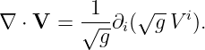
This is the metric divergence formula. It applies beyond orthogonal coordinates.
Figure 6. Divergence compares outward flux through opposite faces of a coordinate cell. The physical face areas and cell volume both involve the metric determinant.
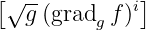
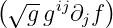
Why this does not require a separate formula for each coordinate systemThe fields V i and the factor
18 Derivation of the Laplace–Beltrami operatorThe scalar Laplacian in Cartesian coordinates is
This geometric definition survives in arbitrary coordinates. The Laplace–Beltrami operator on scalar fields is therefore
We have already derived both ingredients. First, the gradient has contravariant components
Second, divergence is
Replace V i by the gradient components:
This is the central generalization:
The determinant appears because divergence is flux per physical volume; the inverse metric appears because the gradient converts derivatives of a scalar into a vector. Both factors now have physical and mathematical explanations.
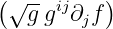
Unpacking both sumsThe notation can be hard to read at first. At a fixed i, the inner sum in Equation (142) is
The outer derivative then acts on that whole expression multiplied by When off-diagonal gij are present, mixed derivatives generally appear. Those terms are necessary in nonorthogonal coordinates.
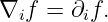
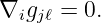
19 Equivalent derivation using Christoffel symbolsThe same scalar operator can be written using a covariant derivative ∇i. For a scalar, the first covariant derivative equals the ordinary partial derivative:
However, the second derivative acts on a covector, so
Here the Levi-Civita Christoffel symbols are
This formula, too, can be derived rather than memorized. The Levi-Civita connection is characterized by two properties: it is torsion free, so Γk ij = Γk ji, and it preserves the metric:
Writing the last condition in components gives
Write two more copies with the indices cyclically permuted:
Add the first two equations and subtract the third. Symmetry of the connection cancels the remaining terms, leaving
Multiply by gkℓ and use gkℓg mℓ = δk m. The result is precisely Equation (146). Thus Christoffel symbols represent the connection uniquely determined by requiring compatible measurements of length and no torsion. These coefficients account for how the coordinate basis changes from point to point. They are built from the metric and its first derivatives. The scalar Laplace–Beltrami operator is the metric trace of the covariant Hessian:
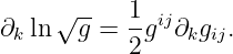
Proving equivalence of the two expressionsThe determinant identity for a differentiable positive-definite matrix is
It follows from differentiating det G by the cofactor formula, or from Jacobi’s determinant rule d(det G) = (det G) tr(G−1dG). Consequently
Contract the Christoffel symbols:
In the second line, the first and third terms cancel after renaming dummy indices and using the symmetry of giℓ and g ik. For a vector, the covariant divergence is
Thus covariant divergence equals the flux-derived divergence in Equation (135). Applying it to V i = gij∂ jf proves that Equations (141) and (152) are equivalent. The key point is that the determinant and inverse metric in Equation (142) already encode the connection terms. One does not need to calculate Christoffel symbols separately to evaluate the scalar Laplace–Beltrami operator.
20 How the Cartesian Laplacian is recoveredFor Cartesian coordinates,
Thus
This reproduces the familiar Cartesian scalar Laplacian.
21 Deriving the cylindrical Laplacian from the metricFrom Equation (94),
with Insert into the Laplace–Beltrami formula:
Since s is independent of ϕ and z, this simplifies to
Check with a Cartesian scalar fieldLet f = x2 + y2 = s2. In Cartesian coordinates,
The same physical scalar result appears in both coordinate descriptions.
22 Deriving the spherical Laplacian from the metricFrom Equation (103),
with
for r > 0 and 0 < 𝜃 < π. Apply Equation (141) term by term:
Move the factors independent of each differentiation outside the derivative:
The r2 and sin 𝜃 factors are not arbitrary calculus decorations: they come from the volume element and inverse metric of the spherical chart.
Check 1: the scalar r2For f = r2,
This agrees with f = x2 + y2 + z2, for which Cartesian differentiation also gives 2 + 2 + 2 = 6.
Check 2: the Cartesian coordinate z = r cos 𝜃Now choose f = r cos 𝜃, which is simply the Cartesian z coordinate. Its Laplacian should vanish. Radial contribution:
Polar contribution:
The azimuthal term vanishes. Hence
The apparently complicated radial and angular parts cancel exactly, as required by coordinate invariance.
23 Laplace–Beltrami on a curved two-dimensional surfaceThe formula is not restricted to three-dimensional volumes. For a two-dimensional surface carrying an induced metric γab,
For a sphere of fixed radius R,
Therefore
This operator differentiates along the surface. It is not the complete three-dimensional spherical Laplacian, because radial differentiation is excluded when r = R is fixed.
A surface eigenfunction calculationTake f(𝜃,ϕ) = cos 𝜃, independent of ϕ. Then
Thus cos 𝜃 is an eigenfunction of the surface Laplacian with eigenvalue −2∕R2. This is the simplest nonconstant example of the eigenfunctions that generalize to spherical harmonics. In electromagnetic theory, spherical harmonics appear in multipole solutions of Laplace’s equation and in wave separation.
24 Nonorthogonal test: Laplace–Beltrami for a shear metricReturn to the nonorthogonal coordinates in Equation (110). The inverse metric is given by
Equation (117), and All metric coefficients are constant, so Equation (141) becomes
Expand the terms:
The mixed derivative −2k∂u∂vf is essential. If we ignored the off-diagonal metric terms, we would get the wrong operator.
Direct independent verificationBecause x = u + kv and y = v, the inverse transformation is
By the chain rule,
Therefore
This agrees exactly with the metric calculation in Equation (189).
25 Physical meaning: electrostatic energy and Poisson’s equationIn Euclidean space, the electrostatic field can be written
Gauss’s differential law is
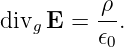
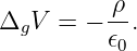
Combining the two equations yields
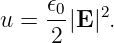
This is Poisson’s equation written in general coordinates. The field equation is the same physics as in Cartesian form, but its differential operator respects the metric. The electrostatic energy density in vacuum is
The squared gradient is
Hence the total energy over a region Ω is
The inverse metric tells us how steep the field is physically, and the metric determinant tells us the physical volume of the region over which that energy is integrated.
26 Integration by parts and the Laplace–Beltrami operatorThe familiar Vector Identity
remains valid geometrically in a Riemannian setting when gradient, divergence, and dot product are interpreted with the metric:
Integrate over a region Ω and apply the divergence theorem with the physical boundary normal:
This is Green’s first identity in metric form, with ∂nh the outward unit-normal derivative. For f = h and boundary conditions making the surface term vanish,
This explains why the Laplace–Beltrami operator, with the convention Δg = div grad, has nonpositive eigenvalues under suitable boundary conditions. Some mathematical texts adopt the opposite sign convention −Δg, so care is needed when comparing references.
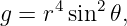
27 Coordinate singularities and genuine geometric curvatureFor spherical coordinates, g = r4 sin 2𝜃 vanishes at the polar axis and at r = 0. For cylindrical coordinates, g = s2 vanishes on the axis. These are failures of the particular coordinate chart: azimuth becomes undefined on an axis, and spherical angles become undefined at the origin. They do not imply that ordinary Euclidean space has become physically singular or curved there. A metric tensor can also describe genuinely curved surfaces or spaces. For example, the induced metric on the sphere has nonzero intrinsic curvature, even though the sphere sits inside ordinary Euclidean three-space. By contrast, the full three-dimensional spherical-coordinate metric describes flat Euclidean space away from its coordinate singularities. The existence of nonzero Christoffel symbols does not by itself prove curvature. Even flat Euclidean space has nonzero Christoffel symbols in polar or spherical coordinates. Curvature is measured by combinations of Christoffel derivatives and products, assembled into the Riemann curvature tensor, which is beyond the core derivation here.
28 What a metric does and does not determineA metric determines lengths, angles, physical area and volume, the Levi-Civita connection, and the scalar Laplace–Beltrami operator on a Riemannian manifold. Appropriate orientation information is also needed to select oriented volume forms and outward normals. The metric does not, by itself, determine charge density, electric potential, or a boundary-value problem’s solution. One still needs the physical field equations, source distributions, boundary data, and, for time-dependent problems, suitable initial data. Nor does the spatial metric alone encode the full spacetime geometry of relativity. In special relativity and general relativity one uses a four-dimensional Lorentzian metric of indefinite signature; the same broad geometric philosophy survives, but signs, time, and causal structure enter the theory.
29 A compact derivation mapThe metric construction can be summarized through the following chain:
For a two-dimensional surface, replace gij by the induced surface metric γab, and use its determinant in both dA and Δγ.
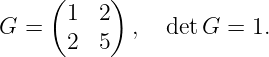
30 Worked review exercise: recover a nonorthogonal metricLet
Then
so
The infinitesimal area is therefore
However, a displacement with du = dv = δ has squared length
A naive Pythagorean sum using only the diagonal metric entries would give 6δ2 and would be wrong. The off-diagonal coefficient measures the essential overlap of the skew directions.
31 Further exercises
References
References
[1] D. J. Griffiths, Introduction to Electrodynamics, 5th ed., Cambridge University Press, 2023. [2] H. M. Schey, Div, Grad, Curl, and All That, 4th ed., W. W. Norton, 2005. [3] M. L. Boas, Mathematical Methods in the Physical Sciences, 3rd ed., Wiley, 2006. [4] G. B. Arfken, H. J. Weber, and F. E. Harris, Mathematical Methods for Physicists, 7th ed., Academic Press, 2013. [5] B. Schutz, Geometrical Methods of Mathematical Physics, Cambridge University Press, 1980. [6] M. P. do Carmo, Differential Geometry of Curves and Surfaces, Prentice Hall, 1976. [7] J. M. Lee, Introduction to Riemannian Manifolds, 2nd ed., Springer, 2018. "The Metric Tensor, Differential Geometry, and the Laplace-Beltrami Operator" is owned by bloftin.
This object's parent. Cross-references: function, delta-function source, Plane polar coordinates, Lorentzian, spacetime, initial data, boundary data, electric potential, charge density, manifold, coordinate singularities, spherical coordinates, Green's first identity, boundary, divergence theorem, Vector Identity, energy, electrostatic field, harmonics, Laplacian, cylindrical coordinates, trace, Cartesian coordinates, unit, flux, vector field, ED03, meridian, volume elements, surface integral, two-dimensional, oriented surface, cross product, Normal, identity, parameters, coordinate systems, square, acceleration, scalar triple product, magnitude, algebraic, determinant, types, work, Kronecker delta, operation, tensor, orthogonal coordinates, regular, commute, matrix, relation, unit vectors, scalar, Einstein summation convention, position, vectors, displacement, position vector, operator, scalar Laplacian, volume, dot product, formulas, ED06, ED02 There are 28 references to this object. This is version 1 of The Metric Tensor, Differential Geometry, and the Laplace-Beltrami Operator, born on 2026-11-20. Object id is 1589, canonical name is MetricTensorDifferentialGeometryAndTheLaplaceBeltramiOperator. Accessed 12 times total. Classification:
|
|
|
|
Pending Errata and AddendaNone.
|
DiscussionNo messages.
|
Interact |












































 into a





























 both change with the chosen coordinate chart, but together
Equation (







 . Finally sum over
 .








 )




 =









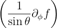










 = 1.














 .
 but the gradient formula contains