Strapdown Inertial Navigation: What a Gyroscope Actually Measures
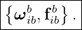
The rotational counterpart to the accelerometer question in INS03 is deceptively simple:
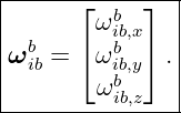
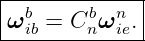
An ideal strapdown rate gyro does not directly measure roll, pitch, yaw, or any other attitude
angle. It measures an angular velocity. With the frame notation established in INS00, the ideal
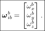
quantity measured by a body-mounted gyro triad is
which means the angular velocity of the body frame b relative to the inertial frame i, resolved in
body coordinates b [1, 2, 3].
This distinction is fundamental. Attitude is an orientation; angular rate is the instantaneous time
derivative of that orientation. A gyroscope therefore provides the rotational input from which a
strapdown navigation computer must propagate attitude.
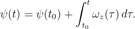
The basic computational chain is
The physics behind the measurement depends strongly on gyro technology. A classical mechanical
gyro uses angular momentum of a rapidly spinning rotor. A MEMS gyro uses the Coriolis response
of a vibrating proof mass. Fiber-optic and ring-laser gyros use the Sagnac effect and
contain no mechanical proof mass at all. Despite these very different mechanisms, all
are designed to estimate the same kinematic quantity: angular rate relative to inertial
space.
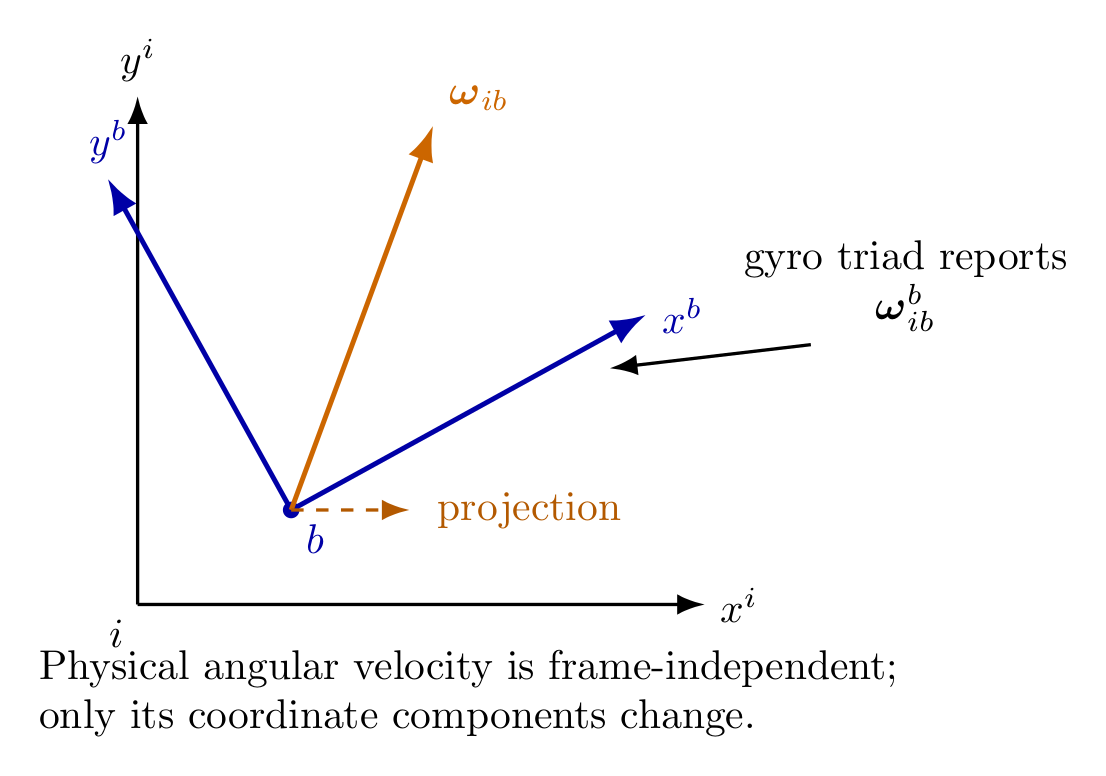
Figure. The body frame b rotates relative to inertial frame i with angular velocity ωib. A
triad of body-mounted gyros resolves this physical angular-velocity vector along the body
axes, producing the components ωibb.
1 Learning objectives
After completing this entry, the reader should be able to:
- distinguish angular velocity from attitude;
- interpret the notation ωibb physically and geometrically;
- explain why a body-mounted gyro can report nonzero angular rate even when a vehicle
appears motionless relative to the Earth;
- derive the torque response of a classical spinning-rotor gyro from angular momentum;
- derive the Coriolis coupling used by a MEMS vibrating-mass gyro;
- explain, at a conceptual level, how optical gyros sense rotation through the Sagnac
effect;
- distinguish the inertial body rate ωibb from the body rate relative to the navigation
frame ωnbb;
- derive the angular-rate decomposition needed by a strapdown attitude mechanization;
- derive the direction-cosine-matrix attitude equation
- explain why a real IMU often supplies angular increments Δ𝜃 rather than an ideal
continuous angular-rate function;
- identify the gyro errors that will be treated quantitatively later in INS18 and INS19.
2 Angular velocity is a physical vector
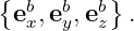
Consider a rigid body carrying an orthonormal body basis
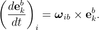
As shown in INS02, if the body rotates relative to inertial space, every body-fixed basis vector
satisfies
The vector ωib is therefore the instantaneous axis and rate of rotation of frame b relative to frame
i.
Its magnitude has units of radians per second,
and its direction is given by the right-hand rule.
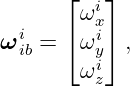
A physical angular-velocity vector can be resolved in any coordinate frame. In inertial
coordinates,
while the same vector resolved in body coordinates is
Because the gyro sensing axes are physically fixed to the vehicle, body coordinates are the natural
output coordinates of a strapdown gyro triad.
3 A gyro measures rate, not orientation
Suppose a vehicle rotates at a constant angular rate about a fixed axis. The gyro can report
that instantaneous rate, but the current attitude depends on the entire history of the
rotation.
For the simplest one-axis case,
Therefore
Even in this scalar case, a gyro measurement alone does not specify ψ unless an initial angle is also
known. In three dimensions the situation is more subtle because rotations about different axes do
not commute. The three gyro channels cannot, in general, be integrated independently as three
scalar Euler Angles. Later entries will derive quaternion and finite-rotation propagation for this
reason.
The essential principle is
4 Classical rotor physics: angular momentum as an inertial reference
The traditional image of a gyroscope is a rapidly spinning wheel or rotor. Although modern
strapdown systems usually use MEMS or optical gyros, rotor physics provides an unusually clear
route to the meaning of an inertial angular-rate sensor [4, 1].
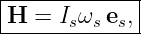
For a symmetric rotor spinning about its symmetry axis with spin rate ωs, the angular momentum
is approximately
where Is is the moment of inertia about the spin axis and es is a unit vector along that
axis.
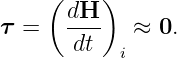
If external torque is negligible,
Hence the angular-momentum direction tends to remain fixed in inertial space even while the
vehicle carrying the gyro rotates around it.
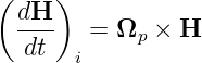
Now suppose the rotor axis is forced to rotate with angular velocity Ωp. Because H is a vector
attached to the rotating rotor axis,
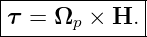
when the spin magnitude is approximately constant. Therefore
This is the basic precession relationship. A torque perpendicular to angular momentum changes
the direction of H rather than simply increasing the spin speed.
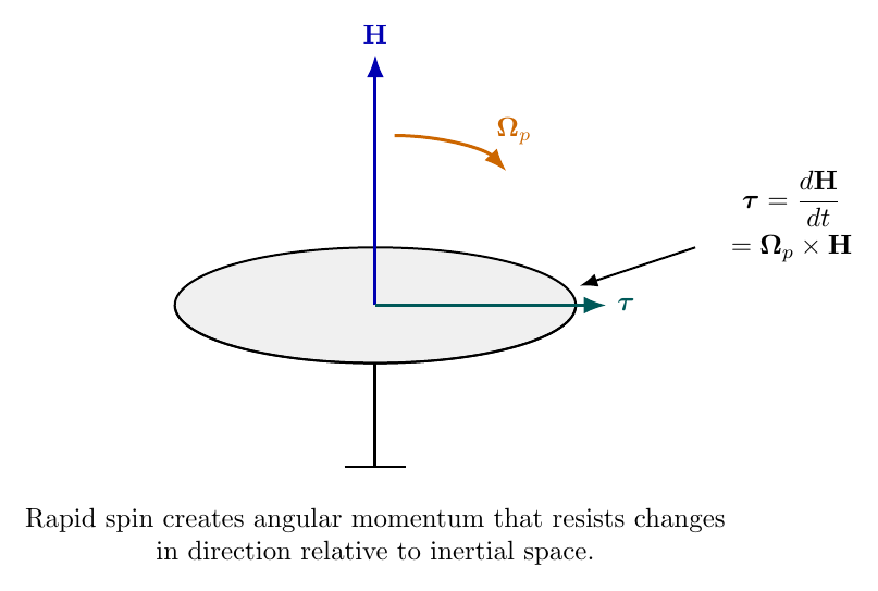
Figure. A rapidly spinning rotor carries angular momentum H. Forcing its axis to precess
with angular velocity Ωp requires a torque τ = Ωp × H. Mechanical gyros exploit this
inertial angular-momentum behavior to sense rotation.
4.1 Why a spinning rotor acts as an inertial reference
The key point is not that the rotor “knows north” or “knows level.” It possesses angular
momentum that resists changes in direction in inertial space. The sensor housing can rotate
relative to that inertial direction, and the relative motion or rebalance torque can be
measured.
Historically, gimbaled inertial systems physically allowed gyro reference elements to remain
approximately inertially fixed while the vehicle rotated around them. In a strapdown system the
sensors are rigidly mounted to the vehicle instead. The navigation computer performs the
coordinate transformations that gimbals once performed mechanically.
5 MEMS gyroscope physics: a vibrating proof mass and Coriolis coupling
A MEMS gyroscope typically contains one or more microscopic proof masses driven into oscillation
along a designated drive direction. When the sensor rotates, Coriolis coupling produces motion or
force along an orthogonal sense direction.
The rotating-frame acceleration equation derived in INS02 contains the Coriolis term
in the inertial-acceleration decomposition. Equivalently, when Newton’s law is written in the
rotating sensor frame, the apparent Coriolis acceleration is
Here vr is the proof mass velocity relative to the sensor structure, and Ω is the rotation rate of
that structure.
Suppose the proof mass is driven along the sensor x axis,
and the sensor rotates about its z axis,
Then
| Ω × vr | = Ωzvd | (20)
|
| = Ωzvdey. | (21) |
Therefore the apparent Coriolis acceleration is
The sensor detects the resulting y-axis displacement or the rebalance force required to suppress
that displacement. In magnitude,
Thus, if the drive velocity is known, the orthogonal response is proportional to the angular rate
Ωz.
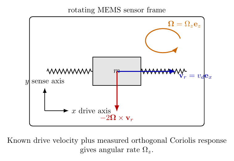
Figure. A MEMS gyro drives a proof mass with velocity vr. Rotation Ω produces a
Coriolis response along an orthogonal sense axis. Measuring the sense displacement or
rebalance force provides an estimate of angular rate.
5.1 A simple driven-mass model
If the sense direction is approximated by a mass-spring-damper system, its displacement y may
satisfy a model such as
with a Coriolis forcing contribution proportional to
The actual electronics demodulate this response using the known drive oscillation. Real devices
require careful treatment of quadrature error, scale factor, bias, damping, temperature, structural
asymmetry, and cross-axis sensitivity. Those error mechanisms belong to INS18. The physics
needed here is simply that rotation converts driven proof-mass velocity into an orthogonal Coriolis
response.
6 Optical gyros: the same quantity without a proof mass
Not all gyroscopes are mechanical. Ring-laser gyros and fiber-optic gyros sense rotation using
counter-propagating light. Rotation changes the effective propagation time around a closed optical
path through the Sagnac effect.
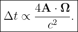
For a loop of area vector A, the leading-order time difference between opposite propagation
directions is proportional to
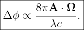
For a single optical loop with wavelength λ, the corresponding phase shift has the form
A fiber coil effectively multiplies the enclosed area by many turns. Ring-laser gyros measure a
rotation-dependent frequency difference between counter-propagating resonant beams. The sensing
physics is different from a rotor or MEMS proof mass, but the estimated kinematic quantity is still
angular rate relative to inertial space.
7 A strapdown IMU uses a gyro triad
A three-dimensional strapdown IMU contains nominally orthogonal gyro sensing axes aligned with
the body axes. With forward-right-down body coordinates,
Each component is a projection of one physical angular-velocity vector onto a body basis
vector:
and similarly for the other two axes.
This is directly analogous to the vector-coordinate distinction developed in INS01. The angular
velocity exists independently of the coordinates used to describe it.
8 A stationary gyro on Earth does not ideally read zero
A common intuition trap is to place an IMU motionless on a table and expect all three gyro
outputs to be zero. The instrument may be motionless relative to the Earth, but the Earth itself
rotates relative to inertial space.
The magnitude of Earth’s rotation rate is approximately
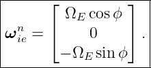
In a local north-east-down navigation frame at geodetic latitude ϕ, the Earth-rate vector is
approximately
The east component is zero because the Earth’s spin axis lies in the local north-down
plane.
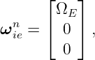
At the equator,
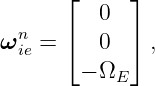
so Earth rate points locally north. At the North Pole,
so it points upward, opposite the positive-down axis.
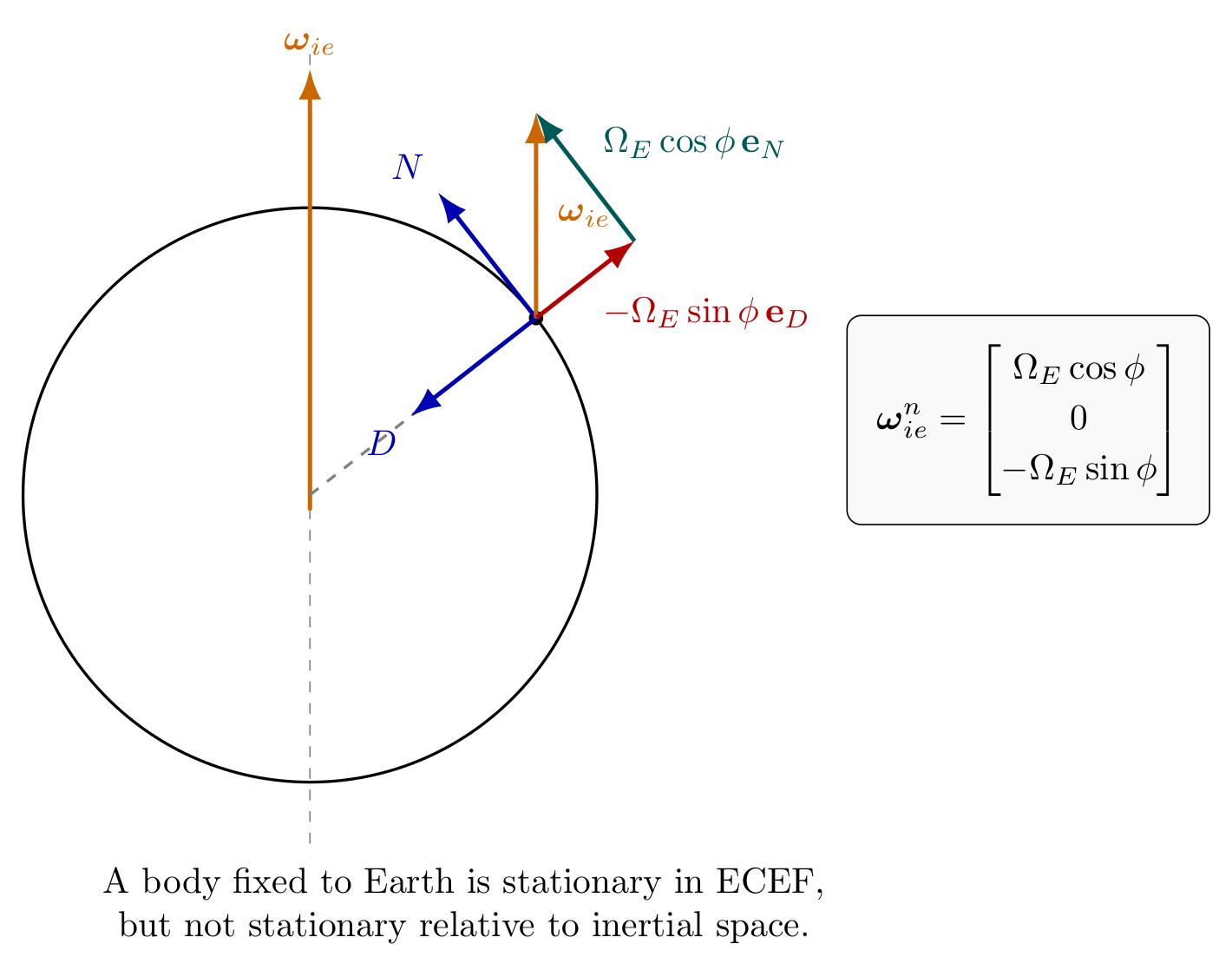
Figure. Earth rotation resolved in a local NED frame. The north component is ΩE cos ϕ,
the east component is zero, and the down component is −ΩE sin ϕ.
If the body is stationary relative to the local navigation frame and the navigation frame is fixed to
the Earth at one location, then ideally
but the gyro still measures Earth rotation:
High-quality inertial gyros can therefore sense Earth rotation. This observation becomes the
physical basis of gyrocompassing and coarse heading alignment in INS09.
9 Which angular rate is needed to update attitude?
The gyro supplies body rotation relative to the inertial frame,
But navigation attitude Cbn describes the body relative to the navigation frame. If the navigation
frame itself rotates relative to inertial space, then the body rate relative to navigation is not
identical to the gyro measurement.
Angular velocities add kinematically. In physical-vector form,
Resolved entirely in body coordinates,
Therefore
This equation explains why “integrate the gyros” is not yet the complete local-navigation
attitude algorithm. The rotation of the chosen reference frame must also be accounted
for.
For a local-level frame on Earth,
The first term is Earth rotation. The second is the transport rate caused by moving the local
navigation frame over the curved Earth. INS06 and INS13 will derive these quantities in
detail.
10 Derivation of the strapdown attitude equation
We now connect the gyro measurement to the direction cosine matrix developed in
INS01.
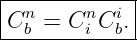
Let
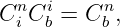
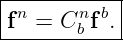
map body-resolved vector components into navigation-resolved components. Insert the inertial
frame as an intermediate frame:
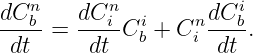
Differentiate using the product rule:
From the rotating-basis result of INS02, a matrix mapping body components into inertial
components obeys
The inverse-direction matrix Cin evolves because the navigation frame rotates relative to inertial
space. Its derivative is
Substitute both identities into the product derivative:
 | = −[ωinn]
×CinC
bi + C
inC
bi[ω
ibb]
×. | (46) |
Since
we obtain
This is one of the central equations of strapdown inertial navigation [1, 2, 5].
The first term rotates the body attitude according to the inertial angular rate measured by the
gyros. The second term compensates for rotation of the navigation frame itself.
11 Equivalent relative-rate form
Using
and the cross-product transformation identity from INS01,
one can show that the attitude equation is equivalently
This form is geometrically intuitive: the body-to-navigation attitude changes according to the
angular velocity of the body relative to the navigation frame.
The inertial-rate form is usually more directly connected to what the gyro measures, while the
relative-rate form makes the geometry especially transparent.
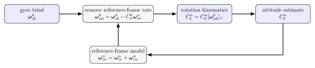
Figure. The strapdown attitude loop. The gyro supplies ωibb. The computed
navigation-frame rate is transformed to body coordinates and removed, leaving ωnbb.
Rotation kinematics then propagate Cbn.
12 Sanity check: pure yaw in an inertial navigation frame
Suppose the navigation frame is inertially fixed,
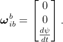
and the body rotates only about its positive z axis with rate  . Then
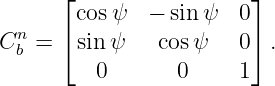
The planar body-to-navigation DCM is
The skew matrix is
Direct multiplication gives
which agrees with differentiating the sine and cosine entries directly. This provides a useful
sign-convention and implementation check.
13 Rate measurements versus angular increments
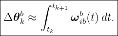
The continuous-time attitude equation is written in terms of angular rate, but a digital IMU
samples over finite intervals. Many inertial instruments provide an integrated angular
increment
At first glance one might expect attitude propagation to consist of simply adding these increments.
That works only in restricted one-axis or infinitesimal cases. Finite three-dimensional rotations do
not commute:
This noncommutativity is the source of coning corrections and is one reason modern strapdown
algorithms propagate quaternions, rotation vectors, or DCMs rather than independently integrated
Euler angles. INS08 will derive quaternion propagation, while INS16 and INS17 will treat sampled
IMU increments, coning, and sculling in detail.
14 Ideal measurement equation and a preview of real gyro errors
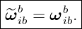
The ideal gyro model is simply
A minimal real-sensor model is
where bg is gyro bias and ng represents measurement noise. More complete models include
scale-factor error, axis nonorthogonality, cross-axis sensitivity, temperature dependence,
g-sensitivity, quantization, bias instability, and other effects.
The present lesson does not yet develop those models. The essential physical consequence, however,
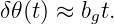
is worth seeing immediately. A constant gyro bias causes attitude error to grow approximately
linearly at first:
INS03 showed that a small tilt error leaks gravity into the horizontal channel,
Therefore a gyro error can become a translational navigation error even if the accelerometers
themselves are ideal. INS19 will derive this error chain quantitatively.
15 Common interpretation mistakes
15.1 Mistake 1: “The gyro measures attitude”
No. It measures angular rate. Attitude must be propagated from rate and an initial
orientation.
15.2 Mistake 2: “A stationary gyro should read zero”
Only if “stationary” means stationary relative to an inertial frame. A body fixed to the rotating
Earth ideally measures Earth rate.
15.3 Mistake 3: “The gyro directly gives body rate relative to NED”
Not exactly. The gyro gives ωibb. For NED attitude propagation one must account for
15.4 Mistake 4: “Integrate each gyro channel to get roll, pitch, and yaw”
That ignores the geometry and noncommutativity of three-dimensional rotation. Euler-angle rates
are not generally equal to the corresponding body-axis gyro rates.
15.5 Mistake 5: “Gyro bias only affects heading”
Bias about any axis creates attitude error. Attitude error rotates specific force incorrectly, so gyro
bias can contaminate velocity and position through gravity and vehicle acceleration.
16 Connection to the complete strapdown mechanization
INS03 established the translational sensor input,
INS04 establishes the rotational sensor input,
Together, the ideal IMU supplies
The gyro data propagate attitude through
and that attitude rotates the accelerometer measurement into navigation coordinates,
The rotational solution therefore sits upstream of the translational solution. An attitude error
immediately becomes a specific-force transformation error.
This is why a strapdown INS is fundamentally a coupled system rather than two unrelated sets of
sensors.
17 Where the series goes next
INS05 will develop gravitation, effective gravity, the rotating Earth, the reference ellipsoid, and
Normal gravity. INS06 will then derive Earth rotation resolved in navigation coordinates and
establish the Earth-fixed and local navigation frames in greater detail.
Later entries will return to the attitude equation developed here:
- INS07 will develop attitude kinematics directly from gyro measurements;
- INS08 will derive quaternion propagation;
- INS09 will use gravity and Earth rate for initial alignment and gyrocompassing;
- INS16 will convert the continuous equations into sampled IMU updates;
- INS17 will derive coning and sculling corrections;
- INS18 will model gyro bias, scale factor, misalignment, and stochastic errors;
- INS19 will derive the resulting navigation error dynamics.
18 Summary
An ideal strapdown gyro measures
body angular velocity relative to inertial space, resolved in body coordinates.
A classical mechanical gyro exploits angular momentum,
with precession governed by
A MEMS gyro uses Coriolis coupling of a driven proof mass,
For navigation, the gyro’s inertial body rate must be distinguished from body rate relative to the
navigation frame:
The resulting DCM attitude equation is
This equation is the bridge from raw gyro measurements to the attitude solution required by the
rest of the strapdown inertial navigation mechanization.
References
[1] David H. Titterton and John L. Weston, Strapdown Inertial Navigation Technology,
2nd ed., Institution of Electrical Engineers, 2004.
[2] Paul D. Groves, Principles of GNSS, Inertial, and Multisensor Integrated Navigation
Systems, 2nd ed., Artech House, 2013.
[3] Christopher Jekeli, Inertial Navigation Systems with Geodetic Applications, Walter
de Gruyter, 2001.
[4] Anthony Lawrence, Modern Inertial Technology: Navigation, Guidance, and Control,
2nd ed., Springer, 1998.
[5] Paul G. Savage, “Strapdown Inertial Navigation Integration Algorithm Design Part
1: Attitude Algorithms,” Journal of Guidance, Control, and Dynamics, vol. 21, no. 1,
pp. 19–28, 1998.
[6] John E. Bortz, “A New Mathematical Formulation for Strapdown Inertial
Navigation,” IEEE Transactions on Aerospace and Electronic Systems, vol. AES-7, no.
1, pp. 61–66, 1971.




![dCn
---b-= Cnb [ωbib]× − [ωnin]×Cnb ;
dt](https://images.physicslibrary.org/cache/objects/1350/make4ht/StrapdownInertialNavigationWhatAGyroscopeActuallyMeasures3x.png)
![|ωib| [rad∕s],](https://images.physicslibrary.org/cache/objects/1350/make4ht/StrapdownInertialNavigationWhatAGyroscopeActuallyMeasures6x.png)



















![|---i------------|
|dC-b i b |
--dt-=--Cb[ω-ib]×.-](https://images.physicslibrary.org/cache/objects/1350/make4ht/StrapdownInertialNavigationWhatAGyroscopeActuallyMeasures43x.png)
![|-------------------|
|dCni-- n n |
| dt = − [ω in ]×C i .|
--------------------](https://images.physicslibrary.org/cache/objects/1350/make4ht/StrapdownInertialNavigationWhatAGyroscopeActuallyMeasures44x.png)
![|---n------------------------|
|dC-b-= Cnb [ωbib]× − [ωnin]×Cnb .
--dt--------------------------](https://images.physicslibrary.org/cache/objects/1350/make4ht/StrapdownInertialNavigationWhatAGyroscopeActuallyMeasures47x.png)

![b n b n n
[C nω in]× = C n[ωin]×C b ,](https://images.physicslibrary.org/cache/objects/1350/make4ht/StrapdownInertialNavigationWhatAGyroscopeActuallyMeasures49x.png)
![|---n--------------|
|dC-b-= Cn[ωb ] .|
--dt------b---nb×--|](https://images.physicslibrary.org/cache/objects/1350/make4ht/StrapdownInertialNavigationWhatAGyroscopeActuallyMeasures50x.png)

![⌊ 0 − dψ 0⌋
b ⌈ dψ dt ⌉
[ω ib]× = dt 0 0 .
0 0 0](https://images.physicslibrary.org/cache/objects/1350/make4ht/StrapdownInertialNavigationWhatAGyroscopeActuallyMeasures55x.png)
![n
dCb-= Cn [ωb ] ,
dt b ib×](https://images.physicslibrary.org/cache/objects/1350/make4ht/StrapdownInertialNavigationWhatAGyroscopeActuallyMeasures56x.png)






![|----------------------------|
|dCnb n b n n |
|-dt--= C b [ω ib]× − [ω in]×C b ,
------------------------------](https://images.physicslibrary.org/cache/objects/1350/make4ht/StrapdownInertialNavigationWhatAGyroscopeActuallyMeasures67x.png)





![|----------------------------|
|dCnb n b n n |
|-----= C b [ω ib]× − [ω in]×C b .
--dt--------------------------](https://images.physicslibrary.org/cache/objects/1350/make4ht/StrapdownInertialNavigationWhatAGyroscopeActuallyMeasures74x.png)