Fourier Series to Fourier Transform

(Topic)

FS26: Fourier Series to Fourier Transform

A Fourier series expresses a periodic function using a discrete list of frequencies. A Fourier transform expresses many nonperiodic functions using a continuous distribution of frequencies. These constructions initially look like different methods. This lecture derives the Fourier transform by watching precisely how a Fourier series changes as its period becomes longer and longer.

The central question is not simply why one sum can be replaced by an integral. We must also understand what happens to the Fourier coefficients, why the frequency spacing appears, where the factor 1∕(2π) comes from, and which assumptions make the limiting argument legitimate.

We follow the PhysicsLibrary progression:

begin with the complex Fourier series from FS18–FS20;
repeat one isolated waveform with an adjustable period T;
derive the connection between discrete coefficients and continuous spectral values;
turn the Fourier series into a Riemann sum and then a Fourier integral;
work a Gaussian wave packet and a rectangular force pulse;
connect the spectrum of a force to the response of a mechanical oscillator.

1 The central contrast: a frequency list and a frequency continuum

A function periodic with period T satisfies

qT(t + T ) = qT(t).

(1)

Its allowed angular frequencies are

ω = nω , ω = 2-π, n ∈ ℤ. n 0 0 T

(2)

The harmonics form a discrete grid. By contrast, a pulse that occurs only once is not characterized by a finite repetition period. Its frequency content need not be limited to this discrete grid.

One way to reveal the connection is to take a single pulse q(t), repeat it every T seconds, and then increase T. The repeated pulses move farther apart. Over any fixed observation interval around the central pulse, the periodic waveform eventually looks exactly like the isolated pulse.

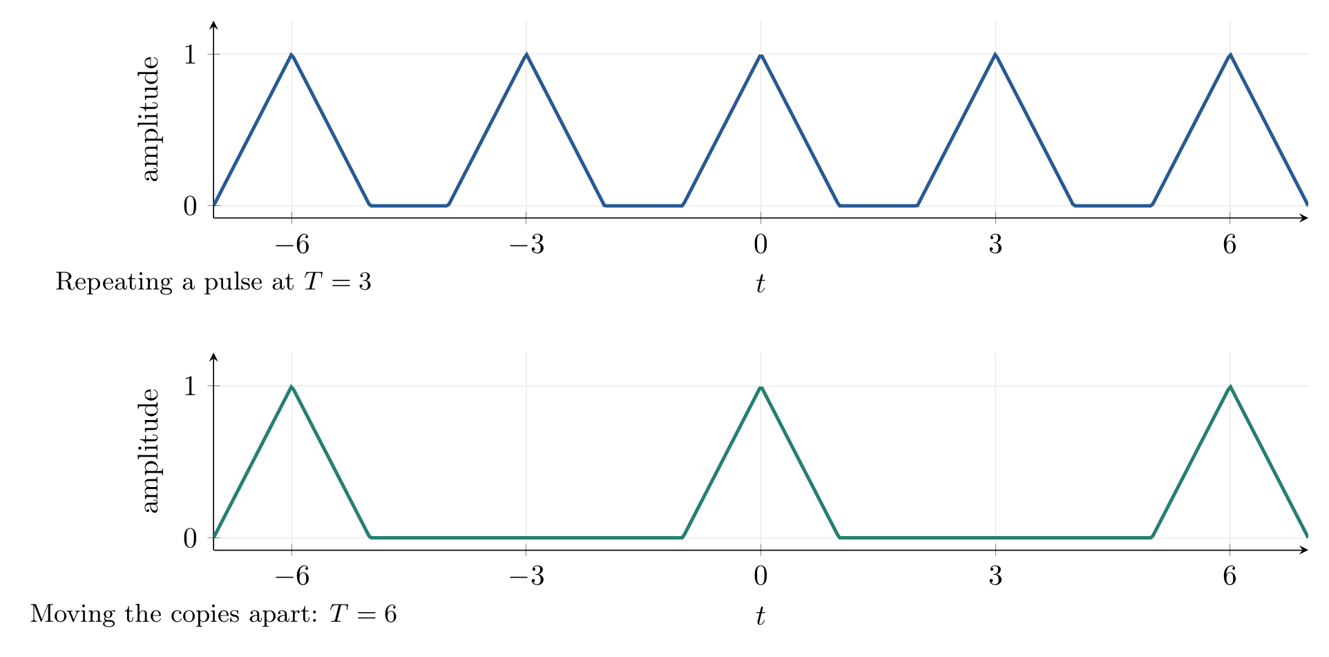
Figure 1. A single localized pulse is repeated at intervals T. Increasing T moves the neighboring copies away. In the limit, a fixed finite time window contains only the central pulse.

2 Recall the complex Fourier series

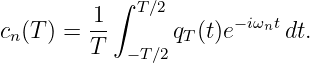
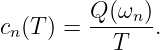
For a T-periodic function that is integrable over a period, its complex Fourier coefficients are

1 ∫ T∕2 cn(T) = -- qT (t)e−iωntdt. T −T∕2

(3)

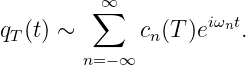
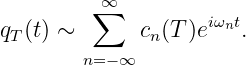
The corresponding Fourier series is

∞ ∑ iωnt qT(t) ∼ cn(T )e . n=−∞

(4)

Here ∼ reminds us that the precise interpretation of equality depends on convergence. Under standard piecewise-smooth assumptions, the series reproduces the function at continuity points and the midpoint of its one-sided limits at a jump.

Why does the coefficient contain 1∕T?

FS02 introduced projection as an inner-product calculation. On one period, the complex exponential basis functions are

iω t ϕn (t) = e n.

(5)

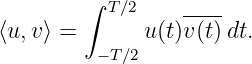
For complex-valued functions, use the inner product

∫ T∕2 ---- ⟨u, v⟩ = −T∕2u (t)v(t)dt.

(6)

Their orthogonality and norms are

⟨ϕn,ϕm ⟩ = T δnm.

(7)

Therefore the projection coefficient of q_T onto ϕ_n is

∫ ⟨qT,ϕn-⟩ 1- T∕2 −iωnt cn = ⟨ϕ ,ϕ ⟩ = T qT(t)e dt. n n −T∕2

(8)

The factor 1∕T comes from the squared norm of a basis function over one period. This is exactly the function-space projection idea from FS02 and FS11.

3 Construct a periodic signal from one isolated waveform

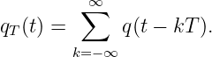
To make the limiting argument transparent, begin with a localized function q(t) that vanishes outside a finite interval [−τ∕2,τ∕2]. Choose T > τ and form its periodic repetition:

∑∞ q (t) = q(t − kT ). T k=−∞

(9)

For any particular t, only finitely many terms can be nonzero, and for T > τ at most one copy contributes. Within the central interval [−T∕2,T∕2], we simply have

qT(t) = q(t).

(10)

This permits us to replace the period integral in Equation (3) by an integral of the original isolated waveform:

c_n(T)	= ∫ _−T∕2^T∕2q(t)e^−iω_nt dt	(11)
	= ∫ _−∞^∞q(t)e^−iω_nt dt.	(12)

No approximation was used in this step. The equality is exact for the compactly supported waveform and T > τ.

This compact-support construction is the simplest teaching route. The resulting transform formulas also apply to many noncompact functions, including Gaussians, with appropriate integrability or limiting arguments.

4 Define the continuous Fourier spectrum

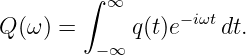
The integral appearing in Equation (12) is a function of the continuous angular frequency ω. Define

∫ ∞ Q(ω ) = q(t)e−iωtdt. −∞

(13)

This is the Fourier transform of q(t) under the angular-frequency convention used in this article.

The continuous variable ω can take any real value. The coefficients of the periodic waveform sample this continuous function only at the allowed harmonic frequencies:

Q(ωn ) cn(T) = ------. T

(14)

It is essential to distinguish the dimensions. If q has units [q] and t is in seconds, then

[Q ] = [q]s, [cn] = [q ].

(15)

A Fourier coefficient has the units of the original waveform. A Fourier transform has those units multiplied by time because it is defined by integration over time.

5 The frequency bins become more closely spaced

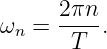
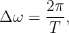
The allowed angular frequencies are

ω = 2πn-. n T

(16)

The difference between adjacent frequencies is

Δω	= ω_n+1 − ω_n	(17)
	= −	(18)
	= .	(19)

Therefore

T −→ ∞ = ⇒ Δ ω −→ 0.

(20)

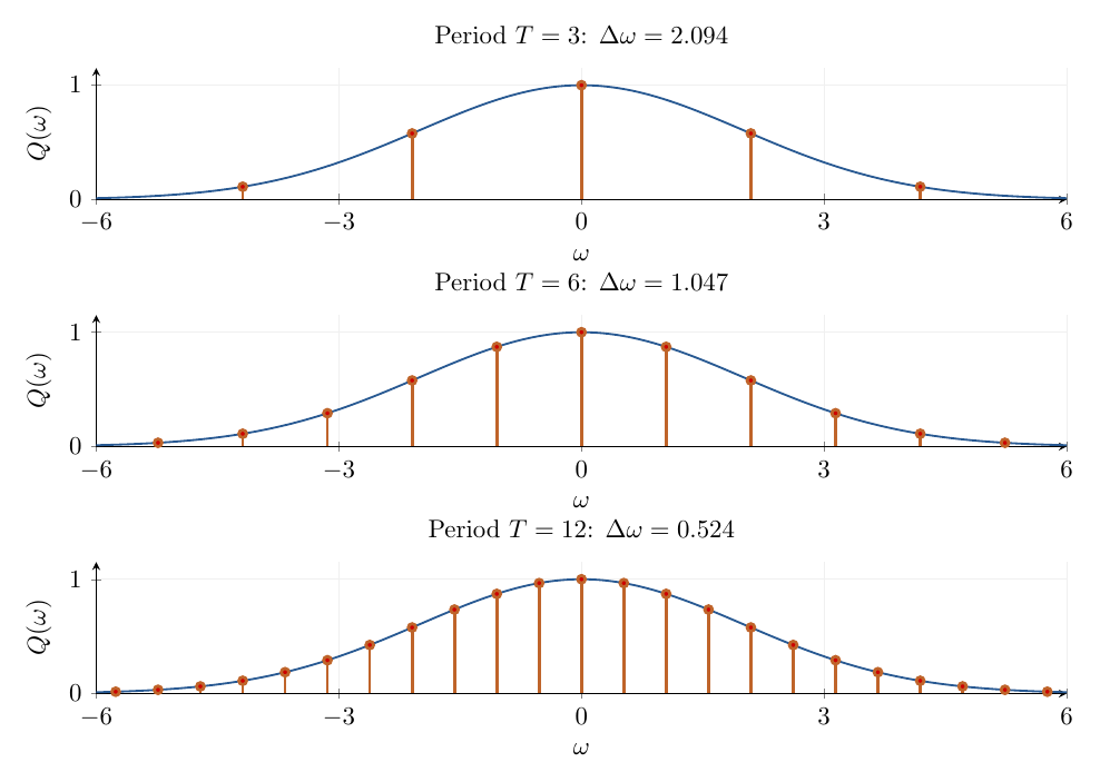
Figure 2. The frequency lattice becomes denser when the repetition period grows. The same smooth spectral envelope is sampled at successively closer frequencies.

The fact that frequencies become dense is not sufficient by itself to derive a Fourier transform. We must also show that the corresponding coefficient Weights have exactly the scaling needed for an integral.

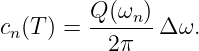
6 The crucial normalization: a coefficient is a bin contribution

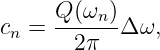
Rearrange Equation (19):

1- = Δ-ω-. T 2π

(21)

Substitute this into Equation (14):

Q(ωn-) cn(T ) = 2 π Δ ω.

(22)

This is the key identity connecting Fourier coefficients to the transform.

The quantity Q(ω_n)∕(2π) plays the role of a frequency-domain density, and Δω is the width of its frequency bin. Their product is the contribution associated with that bin. This is analogous to the Δx weighting that converted a discrete sampled dot product into an integral in FS02.

Because Q(ω_n) remains finite as T grows (for our fixed isolated waveform), an individual coefficient c_n becomes smaller when Δω becomes smaller. That is not signal energy disappearing. More and more frequency bins contribute, with proportionally smaller coefficients.

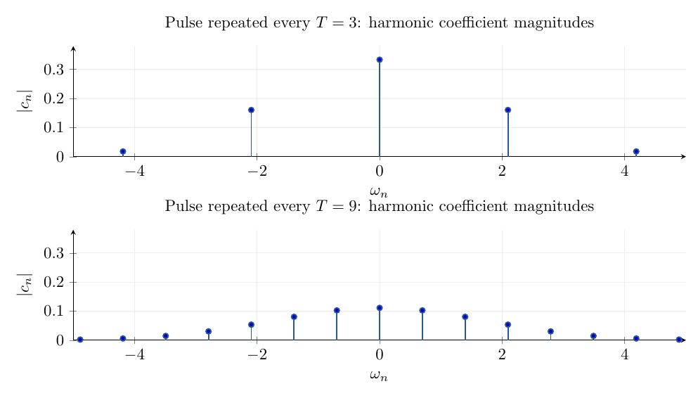
Figure 3. Schematic coefficient magnitudes for a fixed Gaussian-shaped spectrum sampled on two frequency grids. Each coefficient is a spectral value multiplied by the frequency-bin width. At a smaller Δω, each contribution is smaller even though the continuous spectrum has not changed.

7 Derive the inverse Fourier integral from the sum

Start with the complex series:

∞∑ q (t) ∼ c (T )eiωnt. T n n=−∞

(23)

Insert Equation (22):

∞ -1- ∑ iωnt qT(t) ∼ 2π Q(ωn )e Δ ω. n=− ∞

(24)

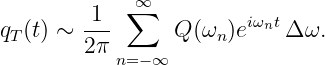
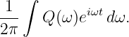
Now look at the right-hand side. It has the familiar structure

∑ (integrand at ωn )(bin width). n

(25)

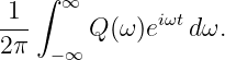
This is a Riemann sum over frequency. As T increases, the grid becomes denser and Δω → 0. Under conditions ensuring the Fourier inversion and the Riemann-sum limit, the right-hand side approaches

∫ ∞ -1- Q(ω )eiωtdω. 2π − ∞

(26)

Meanwhile the periodic copies move away. For a fixed t near the original isolated pulse, q_T(t) = q(t) once T is sufficiently large. We therefore obtain the inverse Fourier transform:

1 ∫ ∞ q(t) = --- Q (ω)eiωt dω. 2π −∞

(27)

Together, Equations (13) and (27) form our Fourier-transform pair.

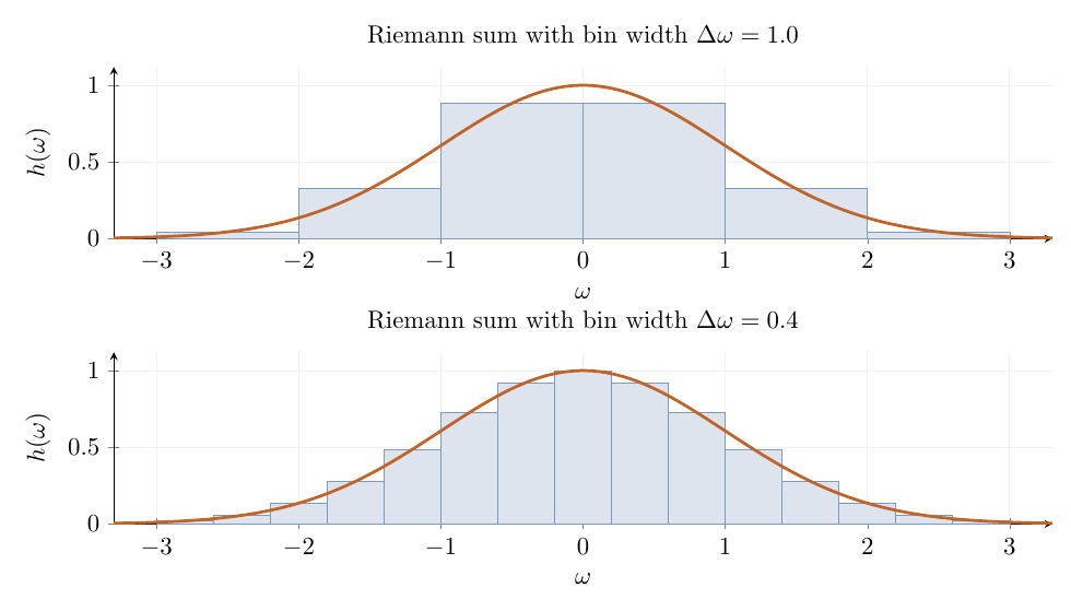
Figure 4. The conceptual sum-to-integral step. Rectangular frequency-bin contributions approximate the area under a spectral integrand; as the bin width tends to zero, the weighted sum becomes an integral. A smooth positive envelope is shown for clarity.

A mathematical qualification about the limit

The preceding derivation is an instructive exact construction through Equation (22), followed by a limiting argument. A rigorous proof must specify the function class and sense of convergence. For sufficiently regular rapidly decreasing functions (for example, Schwartz functions), the transform and inverse integrals have excellent convergence properties. For piecewise-smooth pulses, Fourier inversion at a jump yields the midpoint of the left and right limits. More general L² Fourier inversion requires the language of mean-square limits, as introduced in FS11.

This qualification does not change the frequency-spacing mechanism; it prevents the claim that any arbitrarily pathological function can be reconstructed by manipulating an infinite sum without conditions.

8 What does the Fourier integral mean physically?

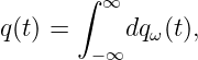
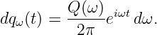
Write the inverse transform in the suggestive form

∫ ∞ q(t) = −∞dq ω(t),

(28)

where a narrow frequency interval contributes approximately

dqω(t) = Q-(ω)eiωtdω. 2π

(29)

A single infinitely narrow frequency interval has an infinitesimal contribution. A finite band contains a finite amount obtained by integrating its contributions.

The exponential e^iωt encodes oscillation at angular frequency ω. The complex value Q(ω) specifies how much of that oscillation is present and its phase relative to the time origin. Fourier analysis changes the question from “what is the waveform doing at time t?” to “what frequencies and phases must be superposed to build the waveform?”

As with Fourier series, the actual waveform is obtained by adding all of these contributions. A real-valued waveform does not require each individual complex term to be real. Positive and negative frequency contributions pair appropriately.

9 Real waveforms, negative frequencies, and phase

If q(t) is real-valued, then

Q(−ω)	= ∫ q(t)e^iωt dt	(30)
	= ∫ q(t)e^−iωt dt	(31)
	= Q(ω).	(32)

This conjugate symmetry guarantees that the positive- and negative-frequency contributions combine to a real function. It also implies that |Q(−ω)| = |Q(ω)|.

If q is real and even, the sine part of the forward transform vanishes, leaving

∫ ∞ Q(ω ) = 2 q(t) cos(ωt )dt. 0

(33)

In that case Q is real and even, although it need not be everywhere positive.

If a waveform is shifted in time,

qt0(t) = q(t − t0),

(34)

then the substitution u = t − t₀ gives

−iωt0 Qt0 (ω ) = e Q (ω).

(35)

The magnitude spectrum does not change, but the phase changes by −ωt₀. This is why magnitude alone cannot usually reconstruct a general waveform.

10 Hertz and radians per second are different transform conventions

Until now ω has measured angular frequency in radians per second. Many engineering and experimental applications prefer ordinary frequency ν in hertz, related by

ω = 2πν, dω = 2π dν.

(36)

Define

∫ ∞ Q (ν) = q(t)e−i2πνtdt. ν −∞

(37)

Then

∫ ∞ q(t) = Q (ν)ei2πνtdν. −∞ ν

(38)

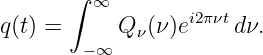
There is no 1∕(2π) in the latter inverse formula. It was absorbed by the variable change dω = 2π dν. The two conventions carry exactly the same information.

Frequency spacing in hertz

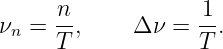
With period T, the ordinary-frequency harmonics are

νn = n-, Δν = 1-. T T

(39)

The periodic coefficient becomes

cn = Q ν(νn )Δ ν,

(40)

so the inverse transform is a direct ν-domain Riemann integral. Confusing ω with ν is one of the most common sources of missing 2π factors.

11 Worked example I: a Gaussian wave packet

Take the smooth localized function

( t2 ) q(t) = A exp − --2- , σt > 0. 2σt

(41)

Here A is its peak amplitude and σ_t sets its time width. It is not compactly supported, but it decays rapidly and its Fourier transform exists as an ordinary absolutely convergent integral.

The forward transform is

∫ ∞ ( 2) Q (ω) = A exp − -t-- e−iωt dt. − ∞ 2σ2t

(42)

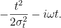
Combine the exponents:

t2-- − 2σ2 − iωt. t

(43)

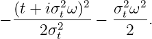
Completing the square gives

(t +-iσ2tω-)2 σ2tω2- − 2σ2 − 2 . t

(44)

Using the standard Gaussian integral (or a corresponding real-variable Fourier-integral derivation), the result is

√ --- ( 2 2) Q (ω) = A σt 2πexp − σtω-- . 2

(45)

The transform of a Gaussian is another Gaussian.

A second derivation using integration by parts

The completed-square argument is concise, but it invokes a Gaussian integral with a complex shift. We can verify the result using only real-variable integration by parts and differentiation under the integral sign.

Write

∫ ∞ I(ω) = g(t)e− iωtdt, g(t) = e−t2∕(2σ2t). − ∞

(46)

Differentiate with respect to the frequency:

∫ ′ ∞ −iωt I(ω ) = − i tg(t)e dt. −∞

(47)

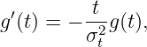
The Gaussian derivative is

g′(t) = − -tg(t), σ2t

(48)

tg (t) = − σ2g′(t). t

(49)

Substitute into the frequency derivative:

∫ ′ 2 ∞ ′ −iωt I(ω ) = iσ t g(t)e dt. − ∞

(50)

Integration by parts gives

∫ _−∞^∞g′(t)e^−iωt dt	= _−∞^∞	(51)
	+ iω ∫ _−∞^∞g(t)e^−iωt dt.	(52)

The boundary term is zero because the Gaussian decays rapidly. Consequently,

I ′(ω) = − σ2ωI (ω). t

(53)

This is a first-order differential equation for the transform. Its solution is

I(ω) = I(0)e−σ2tω2∕2.

(54)

The remaining constant comes from the ordinary real Gaussian integral:

∫ ∞ I(0) = e− t2∕(2σ2t)dt = σ √2-π. −∞ t

(55)

Multiplying by the original amplitude A reproduces Equation (45) with no complex contour argument.

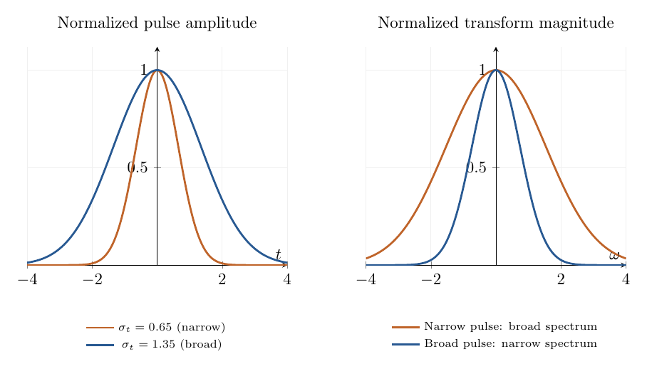
Figure 5. Time- and frequency-domain Gaussian pairs for two pulse widths. A narrower pulse in time has a broader normalized spectrum in frequency, and vice versa. The axes show scaled quantities so the tradeoff is visible.

The essential scale relation is

σ = 1-, ω σt

(56)

where σ_ω is the standard-deviation parameter of the amplitude spectrum Q(ω). This is an illustrative reciprocal-width relation, not yet the general uncertainty theorem. If one uses normalized energy densities |q(t)|² and |Q(ω)|², the corresponding standard deviations instead obey Δt Δω = 1∕2 for this Gaussian.

A dimensional check

If q(t) is measured in volts, then A has units volts, σ_t has units seconds, and Q(ω) has units volt-seconds. The Gaussian-transform prefactor Aσ_t ---
√ 2π therefore has exactly the required units.

12 Worked example II: a rectangular force pulse

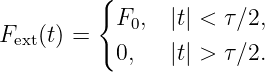
Now consider a force that acts for a finite duration:

{ F0, |t| < τ∕2, Fext(t) = 0, |t| > τ∕2.

(57)

The values at the two endpoints do not affect the transform integral. Here F₀ is a force and τ is the pulse duration.

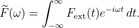
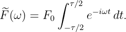
Its Fourier transform is

∫ ∞ ^ − iωt F (ω) = −∞ Fext(t)e dt.

(58)

Because the force vanishes outside the pulse,

∫ ^ τ∕2 −iωt F(ω ) = F0 e dt. −τ∕2

(59)

For ω≠0, integrate directly:

F(ω)	= F₀_−τ∕2^τ∕2	(60)
	= F₀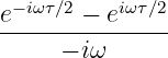	(61)
	= sin .	(62)

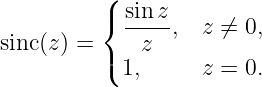
Define the unnormalized-angle sinc function by

( { sin-z- sinc (z) = z , z ⁄= 0, ( 1, z = 0.

(63)

Then

( ) ^ ωτ- F (ω) = F0τ sinc 2 .

(64)

The value at ω = 0 follows by continuity.

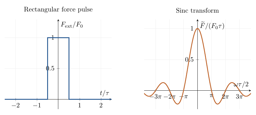
Figure 6. A rectangular force pulse in time has a sinc-shaped spectrum in angular frequency. Longer pulses give narrower spectra; the first zeros occur at ω = ±2π∕τ.

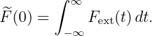
The zero-frequency value is the mechanical impulse

At ω = 0, the exponential kernel equals unity. Therefore

∫ ∞ ^F (0 ) = Fext(t)dt. −∞

(65)

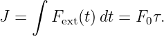
The integral of force over time is impulse:

∫ J = Fext(t)dt = F0τ.

(66)

Thus

^F (0) = J.

(67)

This is a direct connection between Fourier-transform notation and the impulse-momentum theorem. If this is the net force on a constant-mass body, then J = Δp = mΔv.

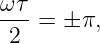
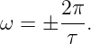
The first nonzero zeros of the force spectrum satisfy

ωτ -2-= ± π,

(68)

ω = ± 2π-. τ

(69)

A shorter duration therefore creates a wider main spectral lobe. If the impulse J is held fixed while τ shrinks, F₀ = J∕τ rises and the spectral width increases. This is one precise mathematical sense in which an impulsive force excites a broad range of frequencies.

A rectangular pulse has nonzero high-frequency tails, so it is not strictly band-limited. This matters for the sampling theorem developed separately in FS26S1.

13 Physics bridge: a force spectrum drives a mechanical oscillator

Fourier transforms also simplify linear differential equations because differentiation in time becomes multiplication by frequency. Consider the damped, driven oscillator

m ¨y(t) + b˙y(t) + ky (t) = F (t), ext

(70)

with m > 0, b > 0, and k > 0. Here y is displacement, b is a damping coefficient, and k is a spring constant.

For a suitably decaying response, integration by parts gives

ℱ {˙y}(ω ) = iωY (ω ),

(71)

2 ℱ {¨y}(ω ) = − ω Y(ω ).

(72)

Transform each term in Equation (70):

(k − m ω2 + ibω )Y (ω ) = ^F (ω ).

(73)

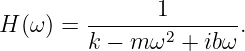
Hence the response transform is

Y (ω) = H (ω )F^(ω ),

(74)

where

-------1------- H (ω) = k − m ω2 + ibω .

(75)

The magnitude of H(ω) indicates which driving frequencies produce a relatively large displacement response. Near the resonant frequency, a lightly damped oscillator responds more strongly than it does at many other frequencies.

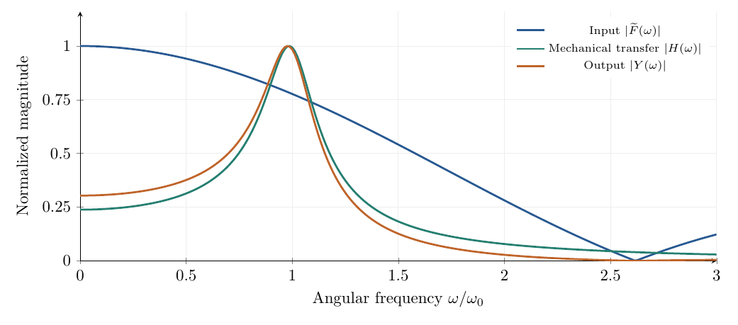
Figure 7. A finite-duration force has a broad input spectrum. A damped oscillator weights those frequency components by its transfer-function magnitude, preferentially responding near its resonance. The curves use illustrative dimensionless parameters.

This is a useful way to interpret the effect of an impact, a vibrating structure, or an acoustic impulse. Instead of solving the time-domain differential equation for every individual waveform, one may transform the forcing, multiply by the response function, and transform back. The formula assumes the stable causal response with no additional separately prescribed homogeneous motion.

14 A periodic sinusoid is a special case, not an ordinary pulse transform

The transform Q(ω) of an isolated integrable pulse is an ordinary function. An infinitely long periodic sinusoid is different: it does not decay at large time, so its Fourier transform is not an ordinary absolutely convergent integral.

For example,

1 1 q(t) = cos(ω0t ) = -eiω0t + -e− iω0t. 2 2

(76)

In the generalized-function (distribution) sense its Fourier transform is

Q (ω) = π δ(ω − ω0) + πδ(ω + ω0 ).

(77)

The two ideal spectral lines are Dirac delta distributions. Their coefficients contain the units necessary to make the inverse transform correct. One should not regard them as two finite-height ordinary samples of a smooth continuous spectrum.

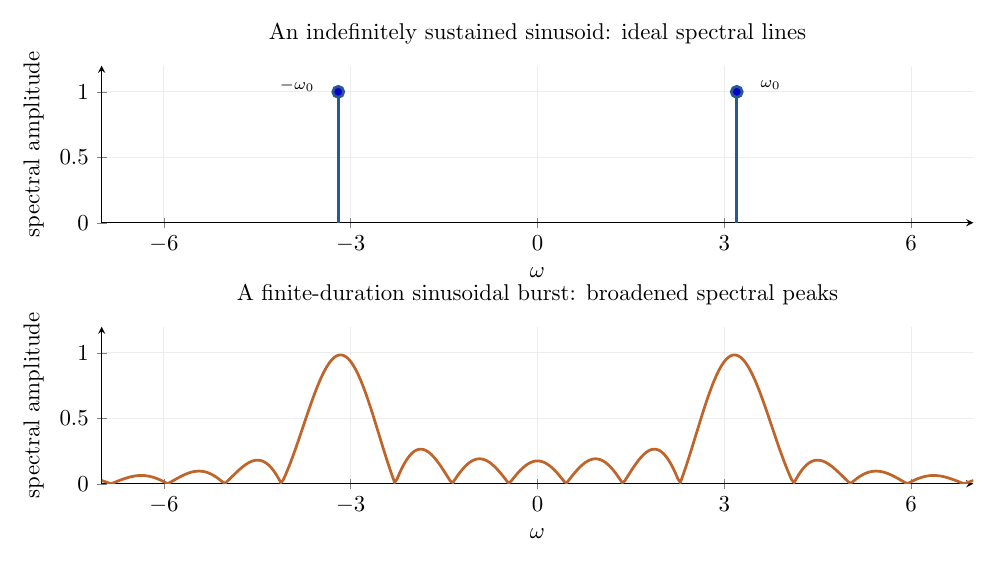
Figure 8. An indefinitely sustained pure tone has spectral lines, represented by Dirac deltas under the continuous transform. A finite-duration windowed tone has a broadened continuous spectrum. The sketches use a fixed angular-frequency convention.

This distinction is central to the physical interpretation of spectra: a perfectly periodic signal is represented by discrete lines, while a localized transient typically requires a continuum of frequencies.

15 Comparison of Fourier series and Fourier transforms


Feature	Fourier series	Fourier transform

Typical signal	periodic q_T(t)	isolated or nonperiodic q(t)
Frequency values	ω_n = 2πn∕T	continuous ω ∈ ℝ
Frequency spacing	Δω = 2π∕T	infinitesimal dω
Spectral information	coefficients c_n	transform Q(ω)
Reconstruction	∑ _nc_ne^iω_nt	(2π)⁻¹ ∫ Qe^iωtdω
Geometry	projection onto discrete harmonics	frequency integral over modes

The table should not suggest that the Fourier transform simply replaces Fourier series in all applications. A genuinely periodic problem is often best analyzed with a Fourier series. A single transient, pulse, or wave packet is naturally described with a Fourier transform. The transform also handles periodic functions when distributions are admitted.

16 Five brief checks with complete answers

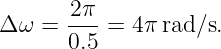
Check 1. Frequency spacing

A waveform is repeated every T = 0.5 s. What is the angular-frequency spacing?

Using Equation (19),

2π Δ ω = --- = 4πrad ∕s. 0.5

(78)

The ordinary-frequency spacing is Δν = 1∕T = 2 Hz.

Check 2. Why coefficients shrink

If the period is doubled, while the isolated pulse itself is unchanged, what happens to each coefficient at a frequency that appears on both harmonic grids?

The transform Q of the isolated pulse does not change. The new coefficient is Q(ω_n)∕(2T) instead of Q(ω_n)∕T, so it is halved. The number of frequency samples per unit bandwidth doubles, preserving the continuum limit.

Check 3. Which normalization belongs in the inverse transform?

With the forward convention Q(ω) = ∫ q(t)e^−iωtdt, the inverse uses

∫ -1- iωt 2π Q(ω )e dω.

(79)

When frequency is in hertz, the inverse uses ∫ Q_ν(ν)e^i2πνtdν. The difference is the change of integration variable, not a physical difference.

Check 4. Force pulse and impulse

A force F₀ = 10 N acts for τ = 0.02 s. Its mechanical impulse is

J = F0τ = 0.20 N s.

(80)

Thus the zero-frequency Fourier transform has value F(0) = 0.20 N s. The first nonzero spectral zeros are at |ω| = 2π∕τ = 100π rad∕s.

Check 5. Why the magnitude spectrum is insufficient

Two time-shifted pulses have identical transform magnitudes because

|Qt0(ω )| = |e−iωt0Q (ω)| = |Q(ω )|.

(81)

Yet they occur at different times. Their phases differ, so both amplitude and phase are generally necessary for waveform reconstruction.

17 Where FS26 fits in the PhysicsLibrary sequence

FS18–FS20 introduced the complex exponential form of Fourier series. FS25 interpreted the discrete harmonic spectrum of a periodic function. FS26 has now shown how the same mathematics becomes a continuous Fourier integral when the repetition period grows and the frequency grid becomes dense.

FS26S1 uses this transform to derive sampling and aliasing: uniform sampling creates repeated copies of a spectrum, and the Nyquist criterion prevents those copies from overlapping. FS27 will use continuous spectra to build localized wave packets and discuss propagation and dispersion.

The essential bridge can be remembered as three equations:

2π Δ ω = ---, T

(82)

Q-(ωn) cn = 2π Δ ω,

(83)

∫ ∑ iωnt ∞ iωt Q (ωn)e Δ ω − → Q (ω )e d ω. n − ∞

(84)

This is the Fourier transform emerging from Fourier series, not as a different trick, but as the natural continuum limit of the same projection and reconstruction ideas.

References

[1] R. N. Bracewell, The Fourier Transform and Its Applications, 3rd ed., McGraw-Hill.

[2] E. M. Stein and R. Shakarchi, Fourier Analysis: An Introduction, Princeton University Press.

[3] A. V. Oppenheim, A. S. Willsky, and S. H. Nawab, Signals and Systems, 2nd ed., Prentice Hall.

[4] G. B. Arfken, H. J. Weber, and F. E. Harris, Mathematical Methods for Physicists, Academic Press.

"Fourier Series to Fourier Transform" is owned by bloftin.
(view preamble)