Forced Wave Equations, Resonant Response, and Modal Green Functions
M06-19 converted the homogeneous wave equation into a spatial eigenvalue problem.
We now add a source.
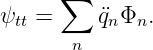
Consider the forced scalar wave equation
The function
represents an external drive.
It may describe:
- a force density on a string or membrane,
- an acoustic source,
- a distributed actuator,
- an idealized impulse,
- a localized point drive.
The crucial simplification is to expand the field in the eigenfunctions of the corresponding
homogeneous boundary value problem.
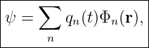
If
with
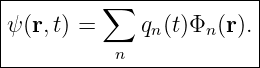
write
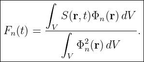
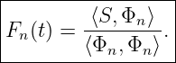
Projection onto one eigenfunction gives
where
Thus a forced wave equation becomes a collection of driven harmonic oscillators.
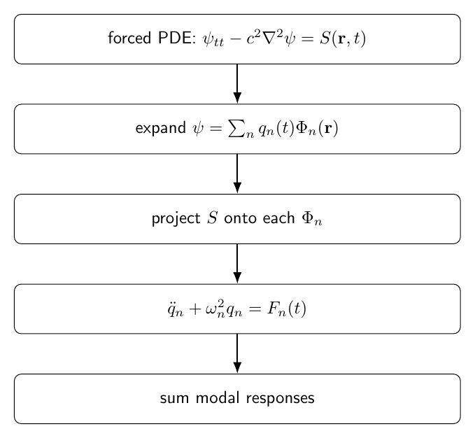
Figure 1. The forcing is projected onto the spatial eigenfunctions. Each modal projection drives
one independent oscillator, and the total field is reconstructed by summing the modal responses.
1 The homogeneous eigenfunctions
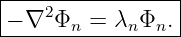
Let the boundary conditions define a self-adjoint spatial problem:
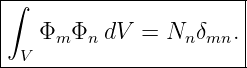
Assume the eigenfunctions are orthogonal:
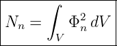
Here
is the mode norm.
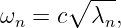
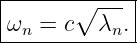
The corresponding natural angular frequency is
2 Modal expansion of the forced field
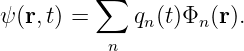
Write
Then
Also,
| − c2∇2ψ | = −c2 ∑
nqn∇2Φ
n | (14)
|
| = c2 ∑
nλnqnΦn | (15)
|
| = ∑
nωn2q
nΦn. | (16) |
Therefore the PDE becomes
3 Projection onto one mode
Multiply by
and integrate over the domain:
| ∑
n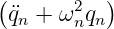 ∫
V ΦmΦn dV | (19)
|
| = ∫
V S(r,t)Φm(r) dV. | (20) |
Using orthogonality,
Thus
where
4 Spatial overlap
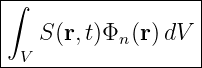
The integral
measures the spatial overlap between the drive and the mode.
A source can strongly excite one mode and fail to excite another even when the forcing frequency
matches both closely.
The temporal frequency controls resonance.
The spatial overlap controls whether the source actually couples to that mode.
These are separate conditions.
5 Localized point forcing
Suppose
Then
| Fn(t) | =  ∫
V δ(r − r0)Φn(r) dV | (26)
|
| =  Φn(r0). | (27) |
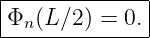
Therefore a point force applied at a node of mode
does not excite that ideal mode:
6 Example 1: center forcing on a fixed string
Consider a string on
with fixed ends.
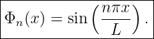
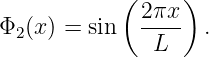
The eigenfunctions are
Apply a point force at
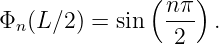
The modal coupling contains
For even
Thus a centered point drive excites only the odd string modes.
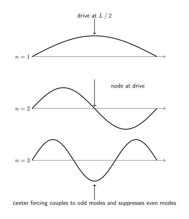
Figure 2. A point drive at the center of a fixed string has zero overlap with every even mode
because those modes have a node at the forcing location.
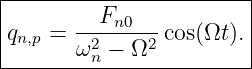
7 Harmonic modal forcing
Suppose one modal force is harmonic:
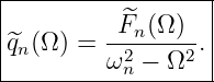
The modal equation is
For
try
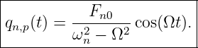
Substitution gives
Therefore
The modal response becomes large when
approaches
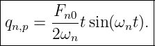
8 Undamped resonance
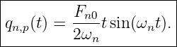
At exact resonance,
the ordinary harmonic trial solution fails because it duplicates the homogeneous solution.
A resonant particular solution is
The oscillation amplitude grows linearly with time.
This does not mean a real physical system develops infinite amplitude.
It means the ideal undamped linear model continuously accumulates energy from a perfectly
phase-matched drive.
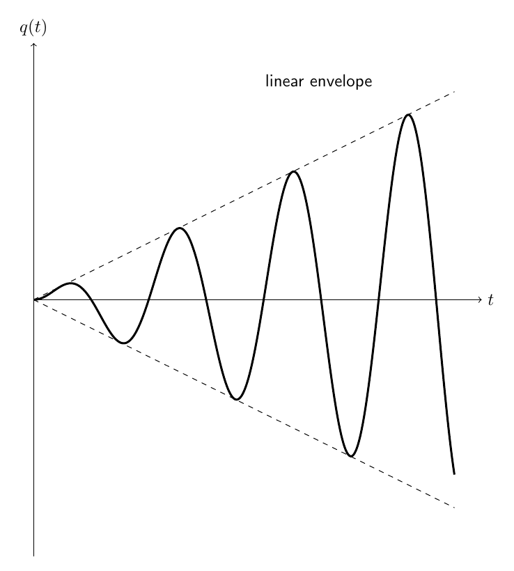
Figure 3. At exact resonance in the ideal undamped model, the envelope grows linearly with time
because the drive adds energy coherently on every cycle.
9 Energy growth at ideal resonance
For
both displacement amplitude and velocity amplitude grow approximately linearly with
Oscillator energy is quadratic in displacement and velocity.
Therefore the modal energy grows approximately as
during ideal exact resonance.
Real damping, nonlinearities, finite source power, or detuning eventually alter this behavior.
10 Adding modal damping
A simple damped modal model is
The coefficient
has units of inverse time.
For harmonic forcing,
the steady-state response can be written
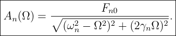
11 Damped steady-state amplitude
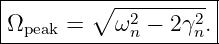
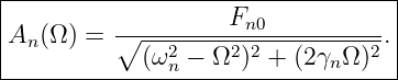
The amplitude is
Damping removes the ideal divergence.
The peak is finite.
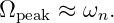
For weak damping, the amplitude resonance occurs near
When
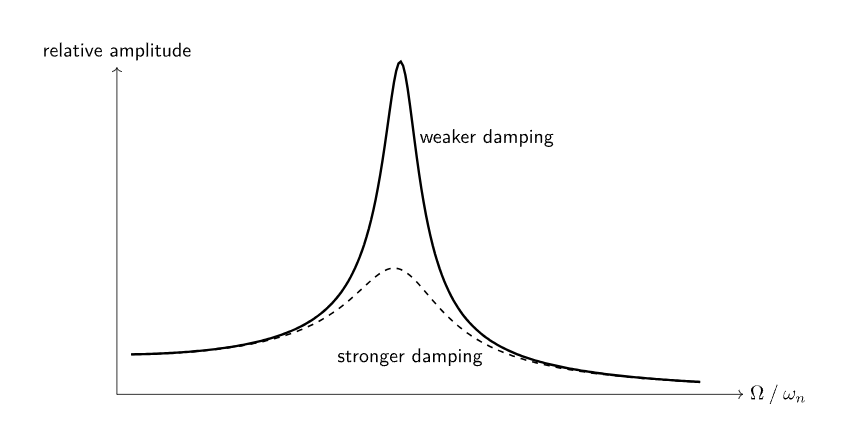
Figure 4. Damping converts the ideal resonance divergence into a finite peak. Smaller damping
produces a taller and narrower resonance curve.
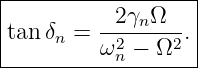
12 Phase lag
The steady-state phase lag satisfies
A quadrant-aware interpretation is required.
At low frequency,
Near resonance,
At high frequency,
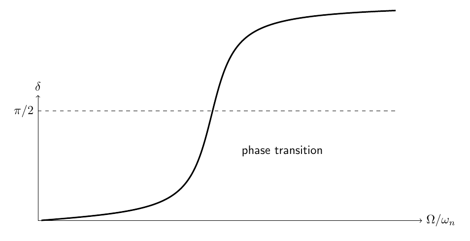
Figure 5. The driven modal response changes from nearly in phase with the drive at low frequency
to nearly opposite phase at high frequency, passing through approximately 90∘ near resonance.
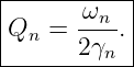
13 Quality factor
For weak damping, define
A large
means:
- weak damping,
- slow free-decay rate,
- narrow resonance,
- large resonant amplification.
For weak damping, the full width at half power is approximately
14 Example 2: resonance width
Suppose
and
Then
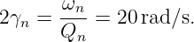
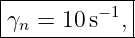
Thus
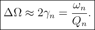
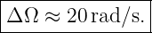
and the weak-damping half-power bandwidth is
15 Impulse forcing
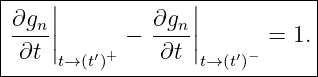
Now drive one modal oscillator with an impulse at time
Integrate the equation
across a very small interval surrounding
The displacement remains continuous, while the velocity jumps:
An impulse therefore gives the mode an instantaneous change in generalized velocity.
16 Retarded modal Green function
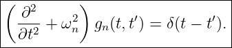
Define
by
The retarded condition requires
For the undamped oscillator,
Here
is the Heaviside step function.
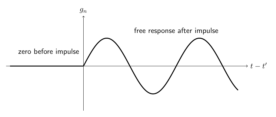
Figure 6. The retarded modal Green function vanishes before the impulse time and then produces
the free sinusoidal response required by the velocity jump.
17 Why the Green function works
For
the function
satisfies the homogeneous equation.
Across
integrating the differential equation gives
The retarded condition makes the derivative before the impulse zero.
The factor
gives exactly the required unit derivative jump.
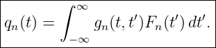
18 Response to an arbitrary modal force
For zero initial conditions,
Because the Green function is retarded,
If forcing begins at
this becomes
This is Duhamel’s principle for one modal coordinate.
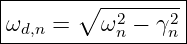
19 Damped modal Green function
For
define
for the underdamped case.
The retarded Green function is
The impulse response now decays with time.
20 Green function for the full wave field
Define the retarded Green function of the wave operator by
It must satisfy the same spatial boundary conditions as the physical field and the retarded
condition
for
Expand
in spatial eigenfunctions.
For nonzero-frequency modes,
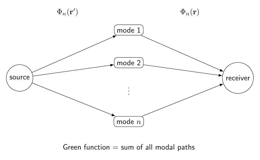
Figure 7. The full retarded Green function propagates a localized source to an observation point
by summing the response of every spatial eigenmode.
21 Field response to a general source
For zero initial conditions,
| ψ(r,t) | = ∫
−∞∞dt′∫
V dV ′ | (96)
|
| × G(r,t; r′,t′)S(r′,t′). | (97) |
Retardation automatically restricts the effective time integration to
The Green function therefore packages:
- the geometry,
- the boundary conditions,
- the normal-mode spectrum,
- causal time evolution.
22 Modal interpretation of source and receiver
In the Green-function expansion, the factor
measures how strongly the source point couples to mode
The factor
measures how strongly that mode appears at the observation point.
Therefore a mode can be suppressed because:
- the source lies at a node,
- the receiver lies at a node,
- both.
This is a useful physical interpretation of modal Green functions.
23 Frequency-domain response
Suppose the forcing varies as
For one undamped modal coordinate,
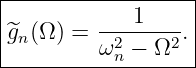
The frequency-domain modal Green function is therefore
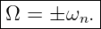
The poles occur at
These poles are the normal-mode resonances.
24 Damped frequency-domain response
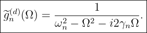
For
with
time dependence,
The poles move away from the real frequency axis.
This mathematical shift corresponds physically to finite decay time and finite resonance
width.
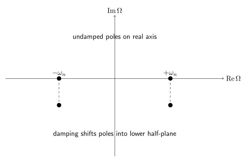
Figure 8. In the ideal system the modal response has real-frequency poles at ±ωn. Damping shifts
the poles off the real axis and produces finite-width resonances.
25 Frequency-domain spatial Green function
For a time-harmonic source at frequency
the field can be expanded as
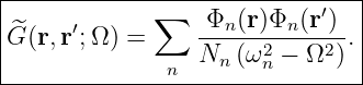
The spatial modal Green function is
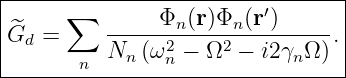
With modal damping,
Near one isolated resonance, the response is often dominated by a single term.
26 Single-mode approximation near resonance
Suppose
is close to one eigenfrequency
and well separated from all others.
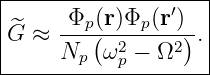
Then
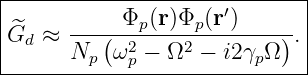
With damping,
This approximation makes the resonant spatial pattern especially clear.
Near resonance, the response looks like the resonant eigenfunction.
27 Example 3: source at a node
Suppose a fixed string is driven harmonically at
The second mode is
At the source,
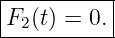
Therefore
Even if the drive frequency is exactly
the ideal centered point drive does not excite mode 2.
Resonance requires both temporal matching and nonzero spatial coupling.
28 Example 4: off-center forcing
Move the string force to
Then
The same mode now couples maximally in this simple normalization.
Thus source placement can qualitatively change the resonance spectrum observed in an
experiment.
29 Uniform forcing and symmetry selection
Suppose a fixed string is driven by a source uniform in space:
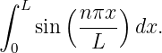
The modal overlap is proportional to
This integral vanishes for even
and is nonzero for odd
Thus a spatially symmetric drive can impose selection rules even without being localized.
30 Green function and initial conditions
The retarded Green function naturally handles forcing with zero initial conditions.
Nonzero initial displacement and velocity may be included by adding the homogeneous
solution
The complete solution is
This separation distinguishes stored initial energy from energy injected by the source.
31 Zero modes require separate treatment
For a Neumann problem, a zero mode may satisfy
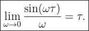
The formula
should then be interpreted by its limit:
Therefore the zero-mode retarded Green function behaves as
Zero modes must not simply be discarded or divided by zero.
32 Causality
A retarded Green function obeys
The response cannot occur before the source acts.
In a finite modal expansion this causality appears through the Heaviside step function.
In unbounded wave propagation, the Green function also contains the travel-time structure
associated with finite propagation speed.
33 Common mistakes
- Expanding the source but not the field in the same eigenfunction basis.
- Forgetting to divide the modal source projection by the mode norm.
- Assuming every source excites every mode.
- Looking only at forcing frequency and ignoring spatial overlap.
- Treating a point source at a modal node as strongly coupled to that mode.
- Using the nonresonant particular solution at exact resonance.
- Interpreting ideal undamped resonant growth as a prediction of infinite real amplitude.
- Forgetting the damping term 2γq.
- Confusing amplitude resonance with the undamped natural frequency when damping
is not weak.
- Using tan δ without selecting the correct phase quadrant.
- Forgetting that Q = ω∕(2γ) for the damping convention used here.
- Omitting the Heaviside factor from a retarded Green function.
- Forgetting the factor 1∕ωn in the undamped impulse response.
- Writing the frequency-domain denominator with the wrong damping sign for the chosen
e−iΩt convention.
- Dividing by ωn for a zero mode without taking the proper limit.
34 Practice exercises
- Starting from the forced wave equation, derive the independent modal equations.
- Derive the modal forcing coefficient for a non-unit orthogonal eigenbasis.
- Show that a point force produces a coupling proportional to the mode value at the
source point.
- Prove that a centered point force on a fixed string excites only odd modes.
- Derive the nonresonant harmonic particular solution for one modal coordinate.
- Derive the linearly growing particular solution at exact undamped resonance.
- Derive the damped steady-state amplitude and phase.
- Starting from Q = ω∕(2γ), derive the weak-damping bandwidth relation.
- Derive the velocity jump caused by an impulse.
- Verify directly that the retarded oscillator Green function has a unit derivative jump.
- Use the Green function to derive the convolution solution for arbitrary modal forcing.
- Derive the underdamped retarded Green function.
- Insert the spatial eigenfunction expansion into the wave-operator Green-function
equation and derive the modal sum.
- Derive the frequency-domain modal denominator for the e−iΩt convention.
- Explain physically why a resonant source placed at a node does not excite that mode.
35 Summary
The forced wave equation is
Using the homogeneous eigenfunctions,
reduces the PDE to
with
For harmonic forcing away from resonance,
At exact undamped resonance,
With damping,
The retarded modal Green function is
The full retarded wave Green function is
Forced wave motion is therefore controlled by three ingredients:
- the modal spectrum,
- the spatial source-mode overlap,
- the temporal response of each driven mode.
References
References
[1] PhysicsLibrary, M06-19, Helmholtz Equation, Boundary-Value Problems, and
Eigenfunction Expansions.
[2] PhysicsLibrary, M06-03, Driven Harmonic Motion and Resonance.
[3] PhysicsLibrary, M06-08, Continuous Strings, Standing Waves, and Normal Modes.
[4] G. B. Arfken, H. J. Weber, and F. E. Harris, Mathematical Methods for Physicists,
7th ed., Academic Press, 2013.
[5] P. M. Morse and H. Feshbach, Methods of Theoretical Physics, McGraw-Hill, 1953.