Deriving IS-GPS-200 Table 20-IV: J2 Gravity and ECEF Satellite Acceleration

1 Where GPSORB15 begins

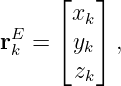
GPSORB13 produced the Earth-fixed satellite position

⌊ x ⌋ E ⌈ k⌉ rk = yk , zk

(1)

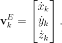
and GPSORB14 produced the corresponding Earth-fixed velocity

⌊ ⌋ ˙xk vEk = ⌈ ˙yk⌉ . ˙z k

(2)

Sheet 4 of IS-GPS-200 Table 20-IV uses these already-computed quantities to obtain

|-----⌊---⌋--| | E ¨xk | |ak = ⌈ ¨yk⌉ .| | ¨zk | --------------

(3)

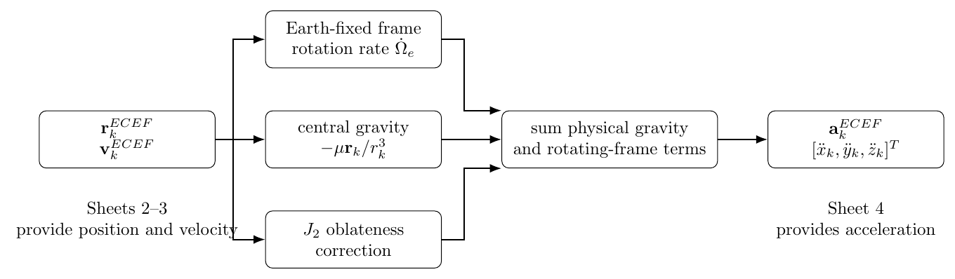
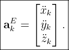
Figure 1. Table 20-IV sheet 4 converts the previously computed ECEF position and velocity into ECEF acceleration.

The official sheet introduces two additional physical constants for this calculation,

|-------------------| RE = 6378137.0 m, | ---------------------

(4)

|-------------------| J = 0.0010826262, | -2-------------------

(5)

and reuses the GPS user values already introduced on sheet 1,

---------------------------- | 14 3 2 | μ-=--3.986005--×-10---m-∕s-,-

(6)

|--------------------------------| |˙Ωe = 7.2921151467 × 10−5 rad∕s.| ----------------------------------

(7)

IS-GPS-200N identifies R_E as the WGS 84 Earth equatorial radius, J₂ as the oblate-Earth gravity coefficient, μ as the GPS user value of Earth’s gravitational constant, and the quantity in Equation (7) as the GPS user value of Earth rotation rate [1].

The current GPS public-document index lists IS-GPS-200N together with later interface revision notices. The derivation below follows Table 20-IV as printed in Revision N; operational software should also review any revision notices applicable to its implementation [2].

2 Step 1: the radius used on sheet 4

The corrected orbital radius from sheet 2 is

rk = A(1 − ecos Ek) + δrk.

(8)

Because the transformation from orbital-plane coordinates to ECEF is a rigid rotation,

|-----∘--------------| | 2 2 2 | -rk =---xk-+-yk-+-zk.-

(9)

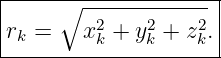
This identity is useful because the acceleration equations are most naturally derived from the Cartesian ECEF coordinates, while the specification writes the scalar distance as r_k.

Define the dimensionless vertical direction cosine

|--------| |qk = zk.| ------rk--

(10)

The repeated factors on sheet 4 can then be recognized as

1 − 5q2k

(11)

and

3 − 5q2k.

(12)

These are signatures of degree-two gravity.

3 Step 2: from spherical gravity to the J₂ potential

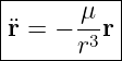
For an ideal spherical Earth, the specific gravitational potential is

μ V0 = − --. r

(13)

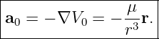
Its gradient gives the familiar central acceleration

|--------------------| |a = − ∇V = − μ-r.| --0--------0-----r3---

(14)

In Cartesian components,

|--------μx--------------μy--------------μz--| |a0x = − -3-, a0y = − -3-, a0z = − -3-.| ---------r---------------r---------------r----

(15)

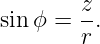
Earth is not spherical. To first order in its axisymmetric departure from spherical symmetry, retain the degree-two zonal term. With geocentric latitude ϕ,

P2 (sin ϕ) = 1-(3 sin2 ϕ − 1), 2

(16)

and

z- sin ϕ = r .

(17)

The potential through J₂ may therefore be written

|-----------------------(---------)--| | μ- μJ2R2E- z2- | |V (r,z) = − r + 2r3 3r2 − 1 .| -------------------------------------

(18)

The first term is spherical gravity; the second is the leading oblateness correction.

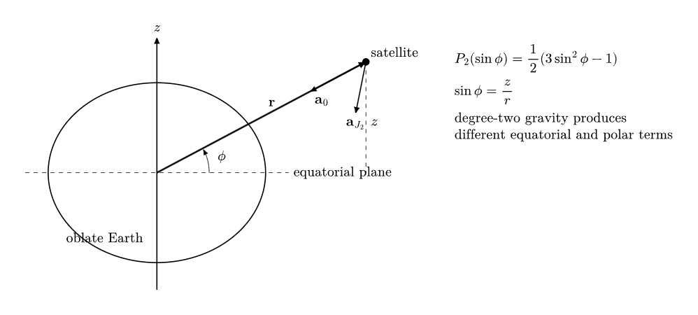
Figure 2. The degree-two gravity correction depends on geocentric latitude through the ratio z/r.

It is convenient to isolate

μJ2R2E- ( 2 −5 −3) VJ2 = 2 3z r − r .

(19)

The acceleration correction is

aJ2 = − ∇VJ2.

(20)

We now differentiate it explicitly.

4 Step 3: derive the Cartesian J₂ acceleration

Since

r = (x2 + y2 + z2)1∕2,

(21)

we have

∂r− m ∂r −m ------= − mxr − (m+2 ), ------= − myr −(m+2), ∂x ∂y

(22)

and

∂r-−m- −(m+2 ) ∂z = − mzr .

(23)

3.1 The x component

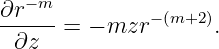
Differentiate Equation (19) with respect to x:

∂V μJ R2 [ ] ---J2 = ---2-E- 3z2 (− 5xr −7) + 3xr −5 . ∂x 2

(24)

Factor the result:

( ) ∂VJ2- 3μJ2R2E--x z2- ∂x = 2 r5 1 − 5r2 .

(25)

Therefore

|--------------------(--------)--| | 3μJ2R2E x z2 | |aJ2,x = − ---------5 1 − 5 -2- .| -------------2----r---------r-----

(26)

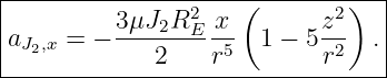
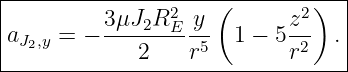
3.2 The y component

By symmetry,

|---------------2----(-------2)--| |aJ ,y = − 3μJ2R-E-y- 1 − 5 z-- .| | 2 2 r5 r2 | ----------------------------------

(27)

3.3 The z component

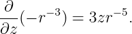
The z derivative requires both explicit and implicit dependence on z:

∂ --(3z2r− 5) = 6zr −5 − 15z3r−7, ∂z

(28)

while

-∂-(− r−3) = 3zr−5. ∂z

(29)

Hence

( ) ∂VJ2- 3μJ2R2E--z z2- ∂z = 2 r5 3 − 5r2 ,

(30)

|---------------2----(-------2)--| |a = − 3μJ2R-E-z- 3 − 5 z-- .| | J2,z 2 r5 r2 | ----------------------------------

(31)

The different coefficients in the horizontal and vertical components are a direct consequence of differentiating the quadrupole potential; they are not ad hoc corrections.

5 Step 4: derive the sheet-4 acceleration factor F

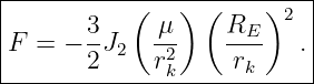
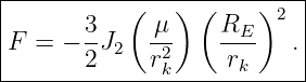
Table 20-IV collects the common dimensional coefficient into

|----------(----)-(----)2--| |F = − 3J -μ RE-- .| | 2 2 r2k rk | ---------------------------|

(32)

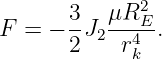
Multiply the factors:

3 μR2 F = − -J2---E4-. 2 rk

(33)

Its dimensions are

m3∕s2- 2 [F ] = m2 = m ∕s .

(34)

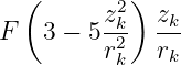
Thus F already has dimensions of acceleration. The remaining bracketed factors in the ICD are dimensionless.

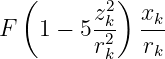
For example,

( ) z2k- xk- F 1 − 5 r2 rk k

(35)

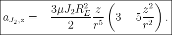
is exactly Equation (26) evaluated at the satellite state. Similarly,

( z2) z F 3 − 5 -k2- -k- rk rk

(36)

is Equation (31).

The negative sign built into F is therefore deliberate. It lets the sheet write the J₂ components compactly without carrying the common factor −3J₂μR_E²∕(2r_k⁴) three times.

6 Step 5: inertial gravity is not yet ECEF acceleration

Central gravity and J₂ describe physical gravitational acceleration. Table 20-IV, however, asks for the second time derivative of coordinates in a rotating Earth-fixed frame. These are not the same thing.

Let I denote an inertial frame and E the Earth-fixed frame. For any vector u,

( ) ( ) du- du- dt = dt + Ωe × u, I E

(37)

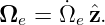
where

Ωe = Ω˙e ˆz.

(38)

Apply Equation (37) first to position:

vI = vE + Ωe × r.

(39)

Differentiate once more. For constant Earth rotation,

|--------------------------------------| |aI = aE + 2Ωe × vE + Ωe × (Ωe × r).| ---------------------------------------

(40)

Solve for Earth-fixed coordinate acceleration:

|--------------------------------------| |aE = aI − 2Ωe × vE − Ωe × (Ωe × r).| ---------------------------------------

(41)

The second term is the Coriolis contribution. The third is the centrifugal contribution. There is no Euler-acceleration term because the user model takes the Earth rotation rate itself as constant.

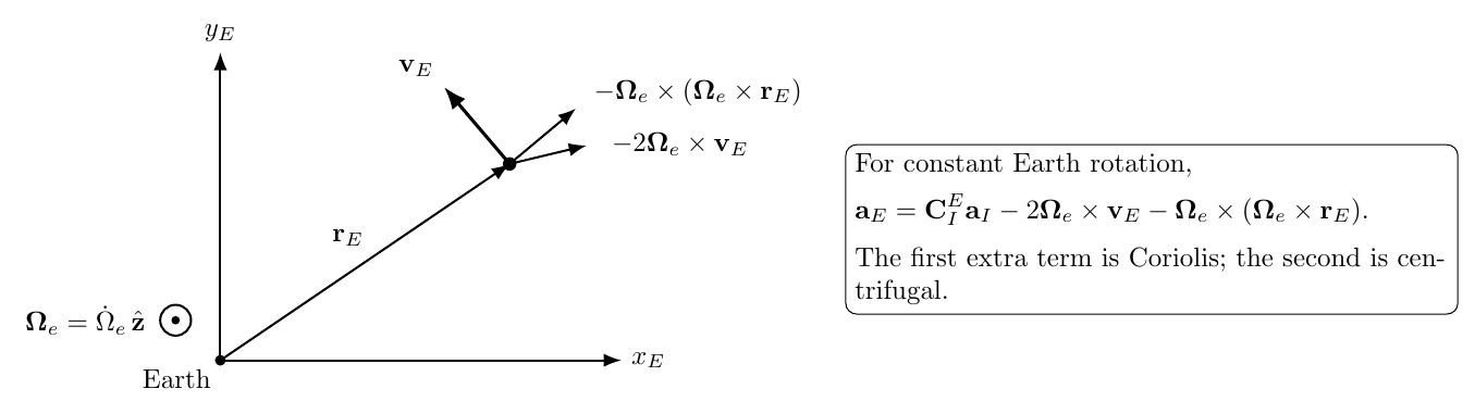
Figure 3. The ECEF second derivative differs from inertial gravitational acceleration by Coriolis and centrifugal terms.

7 Step 6: expand the rotating-frame terms

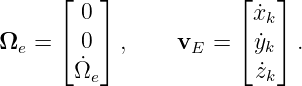
Write

⌊ ⌋ ⌊ ⌋ 0 x˙k Ω = ⌈ 0 ⌉ , v = ⌈y˙ ⌉ . e ˙ E k Ωe ˙zk

(42)

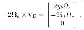
Then

⌊ ⌋ −Ω˙e ˙yk Ωe × vE = ⌈ Ω˙e ˙xk ⌉ . 0

(43)

Therefore

|--------------⌊--------⌋--| | 2y˙k ˙Ωe | |− 2 Ωe × vE = ⌈− 2x˙k ˙Ωe⌉ .| | 0 | ----------------------------

(44)

These are exactly the velocity-dependent terms appearing in the sheet-4 x and y equations.

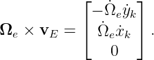
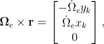
Now compute

⌊ ⌋ − ˙Ωeyk Ωe × r = ⌈ ˙Ωexk ⌉ , 0

(45)

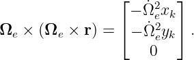
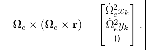
and cross once more:

⌊− Ω˙2 x ⌋ ⌈ e2 k⌉ Ωe × (Ωe × r) = − Ω˙eyk . 0

(46)

Hence

|------------------⌊------⌋--| | Ω˙2exk | |− Ωe × (Ωe × r) = ⌈ Ω˙2 y ⌉ . | e k | -----------------------0-----|

(47)

This explains two visual features of Table 20-IV:

1.: the Coriolis signs are opposite in the x and y equations;
2.: neither Coriolis nor centrifugal acceleration contributes directly to the z equation because the adopted Earth rotation vector is parallel to the ECEF z axis.

8 Step 7: assemble the x acceleration exactly as on sheet 4

The inertial physical acceleration modeled on sheet 4 is

aI = a0 + aJ2.

(48)

Its x component is

[( ( ) ) ] xk- zk- 2 xk- aI,x = − μ r3 + F 1 − 5 r r . k k k

(49)

Add the x entries of Equations (44) and (47):

|----------------[(-------------)----]-----------------| | xk ( zk)2 xk | |¨xk = − μ-3-+ F 1 − 5 --- --- + 2˙ykΩ˙e + xk ˙Ω2e.| ---------rk----------------rk-----rk--------------------

(50)

This is the sheet-4 Earth-fixed x acceleration equation [1].

9 Step 8: assemble the y acceleration

The inertial physical y component is

[( ( )2) ] a = − μ yk-+ F 1 − 5 zk- yk- . I,y r3k rk rk

(51)

The rotating-frame terms now give the opposite Coriolis sign:

|---------------[-(------(---)2-)---]------------------| | yk- zk- yk- ˙ ˙2 | |¨yk = − μr3 + F 1 − 5 rk rk − 2˙xkΩe + ykΩ e.| ----------k--------------------------------------------|

(52)

This is the sheet-4 Earth-fixed y acceleration equation [1].

10 Step 9: assemble the z acceleration

The z component contains central gravity and the distinct vertical J₂ factor,

|---------------[-(------(---)2-)---]--| | zk- zk- zk- | |¨zk = − μr3 + F 3 − 5 rk rk .| ----------k-----------------------------

(53)

No explicit Earth-rate terms appear because the adopted rotation vector has no x or y components. Equation (53) is the final line of Table 20-IV sheet 4 [1].

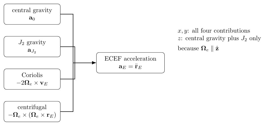
Figure 4. The final ECEF acceleration is the sum of central gravity, J2 gravity, Coriolis, and centrifugal contributions.

11 A compact vector interpretation

The complete sheet may be summarized as

|E-----E----E------------E----------------E---| ak-=--a0-+-aJ2-−-2Ωe-×--vk-−-Ωe-×--(Ωe-×-rk ).-

(54)

This equation is conceptually useful because each term has a distinct origin:

Term	Meaning
a₀	Newtonian inverse-square gravity from a spherical Earth.
a_J₂	Leading correction from Earth’s degree-two oblateness.
−2Ω_e × v_E	Coriolis term caused by differentiating coordinates in the rotating ECEF frame.
−Ω_e × (Ω_e × r_E)	Centrifugal term caused by rotation of the ECEF basis itself.

This form also makes clear that the Coriolis and centrifugal terms are not additional physical forces acting on the satellite in an inertial frame. They appear because the requested acceleration is the second derivative of Earth-fixed coordinates.

12 Numerical continuation of GPSORB12–GPSORB14

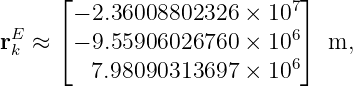
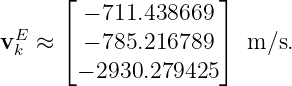
Use the same illustrative satellite state obtained in the preceding articles:

⌊ 7⌋ E − 2.36008802326 × 10 6 rk ≈ ⌈ − 9.55906026760 × 10 ⌉ m, 7.98090313697 × 106

(55)

and

⌊ ⌋ − 711.438669 vE ≈ ⌈ − 785.216789 ⌉ m ∕s. k − 2930.279425

(56)

The radius is

|----------------------------| rk-≈--2.66846771731--×-107-m.--

(57)

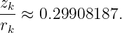
The vertical direction cosine is

zk-≈ 0.29908187. rk

(58)

1. The J2 acceleration factor

Using Equations (4)–(6),

( 14) ( )2 3- 3.986005--×-10--- 6378137- F = − 2 (0.0010826262 ) r2k rk ,

(59)

which gives

|-------------------−5-----2-| -F-≈--−-5.19335-×--10---m-∕s-.|

(60)

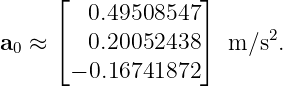
2. Central-gravity contribution

Equation (15) gives

⌊ ⌋ 0.49508547 a0 ≈ ⌈ 0.20052438 ⌉ m ∕s2. − 0.16741872

(61)

Its magnitude is approximately

2 ∥a0∥ ≈ 0.559776 m ∕s .

(62)

3. J2 contribution

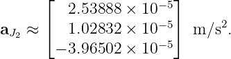
The three J₂ terms are

⌊ − 5⌋ 2.53888 × 10 aJ2 ≈ ⌈ 1.02832 × 10− 5⌉ m ∕s2. − 3.96502 × 10− 5

(63)

The correction magnitude is only about

−5 2 4.82 × 10 m ∕s ,

(64)

but it is systematic and is essential when acceleration is required at navigation accuracy.

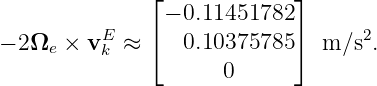
4. Coriolis contribution

Using the ECEF velocity from Equation (56),

⌊ ⌋ − 0.11451782 − 2Ωe × vEk ≈ ⌈ 0.10375785 ⌉ m ∕s2. 0

(65)

5. Centrifugal contribution

Equation (47) gives

⌊ ⌋ − 0.12549755 − Ωe × (Ωe × rEk ) ≈ ⌈− 0.05083025 ⌉ m ∕s2. 0

(66)

6. Final ECEF acceleration

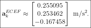
Adding all four contributions gives

|--------------------2-| -¨xk ≈-0.25509549-m-∕s-,-

(67)

|----------------------| |¨yk ≈ 0.25346227 m ∕s2,| ------------------------

(68)

|------------------------| |¨zk ≈ − 0.16745837 m ∕s2.| -------------------------

(69)

Therefore

|---------⌊-----------⌋--------| | 0.255095 | |aECEF ≈ ⌈ 0.253462 ⌉ m ∕s2.| | k | ------------−-0.167458----------|

(70)

Its Earth-fixed coordinate-acceleration magnitude is

∥aECEF ∥ ≈ 0.396685 m ∕s2. k

(71)

This norm should not be confused with the magnitude of inertial gravitational acceleration. ECEF acceleration contains the rotating-coordinate contributions just derived.

For this example the contribution breakdown is

Contribution	x (m/s²)	y (m/s²)	z (m/s²)
Central gravity	+0.49508547	+0.20052438	−0.16741872
J₂ gravity	+0.00002539	+0.00001028	−0.00003965
Coriolis	−0.11451782	+0.10375785	0
Centrifugal	−0.12549755	−0.05083025	0
Final ECEF	+0.25509549	+0.25346227	−0.16745837

13 Physical sanity checks

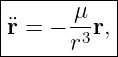
1. Recover Newton’s two-body equation

Set

˙ J2 = 0, Ωe = 0.

(72)

Then F = 0, the rotating-frame terms vanish, and Equations (50)–(53) reduce to

|------μ---| |¨r = − -3r,| -------r----

(73)

which is exactly the Newtonian equation that began GPSORB01.

2. Equatorial point

z = 0,

(74)

then

2 1 − 5(z∕r) = 1,

(75)

so the horizontal J₂ correction becomes

x y aJ2,x = F r-, aJ2,y = F r-.

(76)

Because F < 0, this correction points inward in the equatorial plane.

3. Polar-axis point

x = y = 0, |z| = r,

(77)

then the horizontal corrections vanish and

3 − 5(z∕r)2 = − 2.

(78)

The resulting J₂ vertical correction is outward relative to the central term, reflecting the latitude dependence of the oblate-Earth field.

4. A point stationary in ECEF

vE = 0,

(79)

the Coriolis term disappears but the centrifugal term remains. This is exactly what should happen in a rotating coordinate frame.

5. No direct z-axis rotation terms

Because

Ωe ∥ ˆz,

(80)

Earth rotation does not directly add a z component to either the Coriolis or centrifugal term in this simplified frame model. The entire sheet-4 z equation is therefore gravitational.

14 Why sheet 4 is not a full precision force model

The sheet-4 acceleration model contains

central gravity + J2 + ECEF rotation terms.

(81)

A high-precision orbit propagator may additionally model higher-order geopotential terms, solid-Earth and ocean tides, third-body gravity from the Sun and Moon, solar-radiation pressure, relativistic effects, spacecraft attitude-dependent forces, and maneuvers. Those effects are important to the control segment and to precision orbit determination, but they are not individually reproduced in the compact sheet-4 user equation.

This is consistent with the philosophy developed in GPSORB11: the broadcast ephemeris is a compact user model fitted to a much richer trajectory solution. Sheet 4 provides a useful acceleration consistent with the GPS user-equation framework; it should not be mistaken for the complete force model used to generate the broadcast fit.

15 Implementation checklist

A direct implementation can follow this sequence:

1.: Obtain x_k,y_k,z_k from Table 20-IV sheet 2.
2.: Obtain the three ECEF velocity components from sheet 3.
3.: Compute or reuse r_k = .
4.: Set R_E = 6378137.0 m and J₂ = 0.0010826262.
5.: Compute the factor F from Equation (32).
6.: Evaluate Equations (50), (52), and (53).
7.: Verify units: every term must be in m/s².
8.: During testing, separately log central-gravity, J₂, Coriolis, and centrifugal contributions. Sign mistakes are much easier to find in the decomposed form.

A particularly useful software check is to verify

F < 0

(82)

for positive J₂, μ, R_E, and r_k. Another is to turn off J₂ and Earth rotation independently and confirm the limiting cases described above.

16 The GPSORB derivation chain is now closed

The progression that began with Newton’s law has now reached the complete legacy Table 20-IV state derivatives:

|----------| |¨r = − μ-r | -------r3--|

(83)

led to orbital invariants and conic geometry, then to the six orbital elements, anomaly propagation, the broadcast ephemeris corrections, and finally

|---------------------------ECEF-------ECEF--------ECEF--| -broadcast-parameters-−-→--rk-----−→--vk-----−→--a-k----.|

(84)

The final acceleration model returns directly to dynamics:

|-E------------------------------------------------------| a-k-=-central gravity-+-J2-gravity +-Coriolis-+-centrifugal.

(85)

Thus the four sheets of Table 20-IV are not an isolated collection of formulas. They are the endpoint of the same Newtonian and rotating-frame mechanics developed throughout the GPSORB series.

17 Summary

Table 20-IV sheet 4 begins by defining

|------------------------------------------| R = 6378137.0 m, J = 0.0010826262, | --E----------------------2------------------

(86)

and combines them into

|----------(----)-(----)2--| |F = − 3J -μ RE-- .| | 2 2 r2k rk | ---------------------------|

(87)

This factor comes directly from differentiating the degree-two gravitational potential. The physical gravitational acceleration is then central gravity plus the J₂ correction. Transforming acceleration from an inertial description into the rotating Earth-fixed frame adds

− 2Ω × v e E

(88)

and

− Ωe × (Ωe × rE ),

(89)

which expand into the Coriolis and centrifugal terms printed in the ICD. The resulting component equations are exactly Equations (50)–(53).

References

[1] Global Positioning Systems Directorate, IS-GPS-200N: NAVSTAR GPS Space Segment/Navigation User Interfaces, 1 August 2022, especially Section 20.3.3.4 and Table 20-IV, sheets 1–4. Available from GPS.gov.

[2] GPS.gov, Interface Control Documents (ICDs) and Interface Specifications (ISs), current public-document index, accessed September 2026.

[3] E. D. Kaplan and C. J. Hegarty, eds., Understanding GPS/GNSS: Principles and Applications, 3rd ed., Artech House, 2017.

[4] D. A. Vallado, Fundamentals of Astrodynamics and Applications, 4th ed., Microcosm Press, 2013.

[5] O. Montenbruck and E. Gill, Satellite Orbits: Models, Methods, and Applications, Springer, 2000.

[6] P. D. Groves, Principles of GNSS, Inertial, and Multisensor Integrated Navigation Systems, 2nd ed., Artech House, 2013.

"Deriving IS-GPS-200 Table 20-IV: J2 Gravity and ECEF Satellite Acceleration" is owned by bloftin.
(view preamble)

1 Where GPSORB15 begins

2 Step 1: the radius used on sheet 4

3 Step 2: from spherical gravity to the J2 potential

4 Step 3: derive the Cartesian J2 acceleration

3.1 The x component

3.2 The y component

3.3 The z component

5 Step 4: derive the sheet-4 acceleration factor F

6 Step 5: inertial gravity is not yet ECEF acceleration

7 Step 6: expand the rotating-frame terms

8 Step 7: assemble the x acceleration exactly as on sheet 4

9 Step 8: assemble the y acceleration

10 Step 9: assemble the z acceleration

11 A compact vector interpretation

12 Numerical continuation of GPSORB12–GPSORB14

1. The J2 acceleration factor

2. Central-gravity contribution

3. J2 contribution

4. Coriolis contribution

5. Centrifugal contribution

6. Final ECEF acceleration

13 Physical sanity checks

1. Recover Newton’s two-body equation

2. Equatorial point

3. Polar-axis point

4. A point stationary in ECEF

5. No direct z-axis rotation terms

14 Why sheet 4 is not a full precision force model

15 Implementation checklist

16 The GPSORB derivation chain is now closed

17 Summary

References

3 Step 2: from spherical gravity to the J₂ potential

4 Step 3: derive the Cartesian J₂ acceleration