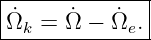
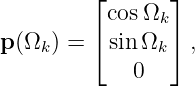
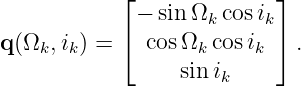
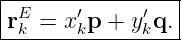
1 Where GPSORB14 begins
GPSORB13 ended with the corrected orbital quantities
the node-aligned orbital-plane coordinates
and the Earth-fixed coordinates
IS-GPS-200 states that a user can compute satellite velocity and acceleration, if required, using the
equations in parts 3 and 4 of Table 20-IV. Sheet 3 is therefore best understood as the analytical
time derivative of the complete sheet-2 position chain [1].
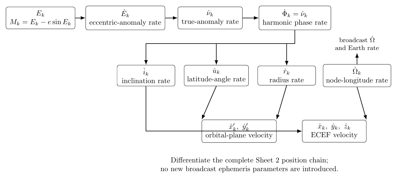
Figure 1. Sheet 3 differentiates the complete Sheet 2 position chain to produce ECEF velocity.
The current GPS public-document index lists IS-GPS-200N as the base L1/L2 interface
specification, together with later interface-revision notices. This article derives the Table 20-IV
sheet-3 equations as printed in Revision N; operational software should also review any applicable
current revision notices [2, 1].
2 A local time derivative and the ephemeris time offset
The sheet-1 time variable is
with the beginning/end-of-week correction applied so that it represents the actual time difference
to the ephemeris reference epoch. Within one continuous evaluation interval,
This seemingly trivial fact is used repeatedly below. A software implementation should not
numerically differentiate across an artificial week-wrap discontinuity; the physical orbit itself is
continuous.
The quantities A, e, Δn, ω, the six harmonic coefficients, i0, IDOT, Ω0, and the transmitted
node-rate parameter are treated as constants over the broadcast fit interval. Their purpose is to
parameterize the fitted trajectory over that interval, not to become new dynamical states at every
evaluation time.
3 Step 1: eccentric-anomaly rate
GPSORB12 solved Kepler’s equation
The broadcast mean anomaly is
where
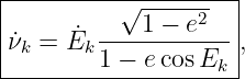
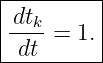
Because n is constant over the evaluation interval and Equation (7) gives dtk∕dt = 1,
Differentiate Equation (8):
Factor the eccentric-anomaly rate:
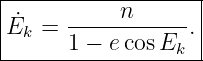
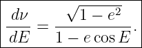
Substitute Equation (11) and solve for the eccentric-anomaly rate:
This is the first equation on Table 20-IV sheet 3 [1].
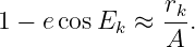
The denominator has a familiar geometric meaning because
Thus, ignoring the small broadcast radius correction,
Near periapsis this factor is smaller, so eccentric anomaly advances faster; near apoapsis it is
larger, so eccentric anomaly advances more slowly.
4 Step 2: true-anomaly rate
GPSORB12 used the quadrant-safe relation
To differentiate it cleanly, define
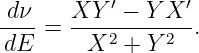
For an angle
the derivative is
Now
The numerator of Equation (20) becomes
so
The denominator is
which simplifies to
Therefore
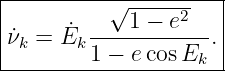
Applying the chain rule,
This is the sheet-3 true-anomaly-rate equation [1].
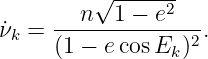
Combining Equations (14) and (27) also gives
This agrees with Kepler’s second law: angular motion is faster when the satellite is closer to
Earth.
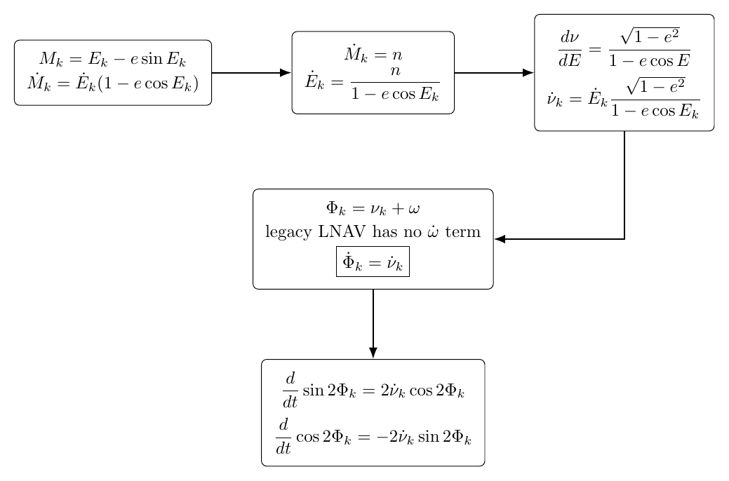
Figure 2. Differentiating Kepler’s equation and the eccentric-to-true-anomaly mapping produces
the phase rates used by the harmonic corrections.
5 Why the harmonic phase rate equals the true-anomaly rate
The uncorrected argument of latitude is
In a complete perturbation theory, the osculating argument of periapsis generally has a nonzero
rate. GPSORB10 derived the familiar secular J2 apsidal precession as one example. The legacy
LNAV user model, however, does not transmit a separate argument-of-periapsis-rate
term in this calculation. The fitted parameter ω is treated as constant while the other
broadcast rates and harmonic coefficients absorb the required short-interval trajectory
behavior.
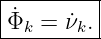
Hence, within this prescribed user model,
That identity explains why every harmonic derivative on sheet 3 contains twice the true-anomaly
rate.
6 The common derivative behind all three harmonic channels
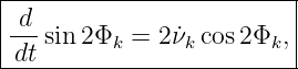
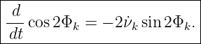
The sheet-2 corrections depend on sin 2Φk and cos 2Φk. Their time derivatives are
and
Using Equation (30),
The factor of two is not an arbitrary GPS convention. It is the chain-rule derivative of the
twice-per-revolution phase 2Φk.
7 Step 3: corrected inclination rate
GPSORB13 used
where
Differentiate Equation (35):
Using Equations (33) and (34),
Therefore
This is the corrected inclination-angle rate on sheet 3 [1].
The first term is the fitted linear inclination drift; the second is the instantaneous slope of the
twice-per-revolution inclination correction.
8 Step 4: corrected argument-of-latitude rate
The corrected argument of latitude is
with
Differentiate:
Because the harmonic phase rate equals the true-anomaly rate,
Thus
The first term is the idealized in-plane angular rate. The second term is the rate contributed by the
fitted harmonic correction.
9 Step 5: corrected radius rate
The corrected radius is
where
Differentiate the Keplerian part first:
Next,
Therefore
The units provide a useful check: the first term is meters times radians per second, where radians
are dimensionless, and the second term is meters times radians per second. Both are meters per
second.
10 Step 6: Earth-fixed node-longitude rate
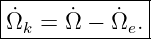
GPSORB09 and GPSORB13 derived
Here the first rate on the right-hand side is the transmitted node-rate parameter, while the second
is the prescribed Earth rotation rate. Differentiate Equation (50). The reference quantities are
constant over the fit interval, so
This is the sheet-3 longitude-of-ascending-node rate [1].
For a GPS-like satellite, the magnitude of the Earth-rate term is much larger than the small
inertial node-precession rate. That is expected because Ωk is an Earth-fixed longitude, not an
inertial right ascension.
11 Step 7: orbital-plane velocity
Differentiate the sheet-2 orbital-plane coordinates from Equation (2). For the first component,
Hence
For the second component,
These are the in-plane velocity equations printed on sheet 3 [1].
They are also the Cartesian expansion of the familiar polar-coordinate velocity
The two terms have clear physical meanings:
- the first term is the radial velocity;
- the second term is the transverse velocity.
Because the local basis vectors are orthonormal,
This provides a convenient numerical check on Equations (53) and (54).
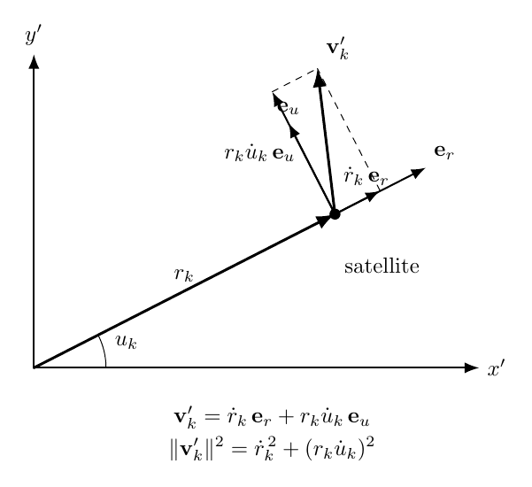
Figure 3. Orbital-plane velocity is the vector sum of radial motion and transverse motion.
12 Step 8: derive the final ECEF velocity by the product rule
The cleanest way to understand the final three equations is to rewrite the sheet-2 ECEF position
in terms of two time-varying basis vectors. Define
and
Then Equations (3)–(5) can be written compactly as
Differentiate using the product rule:
This equation separates three sources of ECEF velocity:
-
1.
- motion within the corrected orbital plane through the two in-plane velocity
components;
-
2.
- Earth-fixed node sweep through the node-longitude rate;
-
3.
- change in the corrected inclination through the inclination rate.
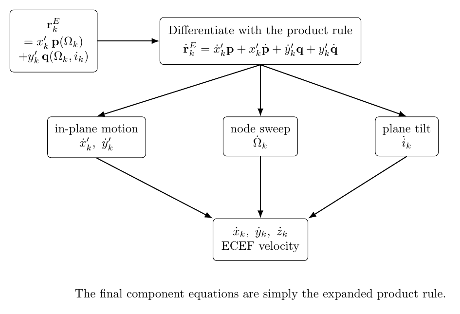
Figure 4. The final ECEF velocity equations are the product-rule derivative of the time-varying
orbital-plane basis.
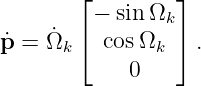
The derivative of p is
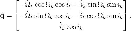
For q, differentiate both Ωk and ik:
Substituting Equations (61) and (62) into Equation (60) and reading off the components gives the
three sheet-3 ECEF velocity equations.
ECEF x velocity
Define the basis-rate combination
Then
ECEF y velocity
Define
Then
ECEF z velocity
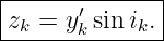
These expressions are exactly what should emerge from differentiating the sheet-2 position
equations. They are not an independent velocity model.
13 Why the ECEF speed is not the inertial orbital speed
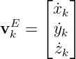
The vector
is a coordinate velocity in the rotating Earth-fixed frame. It should not be confused with the
inertial speed from vis-viva. In general,
so Earth rotation changes the numerical components and the norm of the coordinate velocity. This
is the same rotating-frame physics introduced in GPSORB09.
14 Numerical continuation of GPSORB12–GPSORB13
Continue the previous example with
and the same harmonic coefficients used in GPSORB13:
Also retain
with
GPSORB13 already obtained
and
1. Eccentric-anomaly rate
Equation (14) gives
2. True-anomaly rate
Equation (27) gives
3. Corrected inclination rate
Using Equation (39),
The harmonic contribution is therefore small compared with the orbital angular rate, as
expected.
4. Corrected argument-of-latitude rate
Equation (44) gives
5. Corrected radius rate
Equation (49) gives
The radial speed is much smaller than the transverse speed, which is typical for a low-eccentricity
GPS orbit.
6. Earth-fixed node-longitude rate
so
7. Orbital-plane velocity
Equations (53) and (54) give
The in-plane speed is
Equation (56) independently gives
confirming the orbital-plane differentiation.
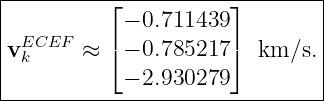
8. Final ECEF velocity
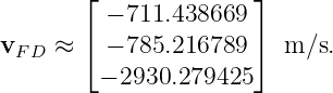
Substituting the position, angle, and rate quantities into Equations (64)–(67) gives
Therefore
Its ECEF speed is
The smaller norm compared with the roughly 3.86 km∕s orbital-plane speed is not a contradiction;
ECEF is a rotating coordinate frame.
15 Finite-difference verification
A powerful implementation test is to compare the analytical velocity against a central difference of
the full position algorithm. Let
Using the complete sheet-1 and sheet-2 algorithm with h = 0.1 s for the numerical example gives
approximately
The norm of the difference from the analytical result is below
for this example. This is an excellent unit test because it validates the chain rule, harmonic signs,
node-rate sign, and final ECEF product rule simultaneously.
16 Sanity checks that catch common receiver bugs
Circular-orbit limit
If e = 0, then
and Equation (27) reduces to
If the radial harmonic coefficients also vanish,
Zero-harmonic limit
If
then
and
These are the expected derivatives of the uncorrected broadcast orbit.
In-plane speed identity
After computing the two orbital-plane velocity components, verify
A discrepancy usually indicates a sign error in one of the product-rule terms.
Differentiate the final position numerically
For a test ephemeris, evaluate the full ECEF position at t−h, t, and t + h and compare the central
difference with Equations (64)–(67). This is one of the most effective end-to-end checks of a
broadcast-ephemeris implementation.
17 Implementation sequence
A direct implementation of Table 20-IV sheet 3 can follow this order:
-
1.
- Reuse n, Ek, νk, Φk, uk, rk, ik, x′k, y′k, and Ωk from sheets 1 and 2.
-
2.
- Compute the eccentric-anomaly rate using Equation (14).
-
3.
- Compute the true-anomaly rate using Equation (27).
-
4.
- Compute the corrected inclination rate using Equation (39).
-
5.
- Compute the corrected argument-of-latitude rate using Equation (44).
-
6.
- Compute the corrected radius rate using Equation (49).
-
7.
- Compute the node-longitude rate using Equation (51).
-
8.
- Compute the two orbital-plane velocity components using Equations (53) and (54).
-
9.
- Compute the three ECEF velocity components using Equations (64)–(67).
-
10.
- Verify the in-plane speed identity and, during testing, compare with a central difference
of the position algorithm.
All angular quantities used inside trigonometric functions and angular-rate equations must be in
radians and radians per second after any required conversion from the broadcast semicircle
representation.
18 Connection to the next sheet
Sheet 3 closes the loop from broadcast orbit parameters to ECEF position and velocity:
Table 20-IV sheet 4 then moves from kinematics back to dynamics. It supplies an ECEF
acceleration model containing central gravity, the J2 oblateness correction, and the Coriolis and
centrifugal terms associated with the rotating Earth-fixed frame [1]. That next step reconnects
the GPS user algorithm directly to the Newtonian equation that began the GPSORB
series.
19 Summary
The sheet-3 velocity equations are not a separate set of empirical formulas. They are the analytical
derivative of sheets 1 and 2. The essential chain is
then
followed by
These rates generate the in-plane velocity through
and differentiating the time-varying Earth-fixed basis then gives the three ECEF velocity
components.
The next article can derive Table 20-IV sheet 4: the J2 acceleration factor, Earth-fixed
gravitational acceleration, Coriolis acceleration, centrifugal acceleration, and the final ECEF
acceleration equations.
References
[1] Global Positioning Systems Directorate, IS-GPS-200N: NAVSTAR GPS Space
Segment/Navigation User Interfaces, 1 August 2022, especially Section 20.3.3.4 and Table
20-IV, sheets 1–4. Available from GPS.gov.
[2] GPS.gov, Interface Control Documents (ICDs) and Interface Specifications (ISs),
current public-document index, accessed September 2026.
[3] E. D. Kaplan and C. J. Hegarty, eds., Understanding GPS/GNSS: Principles and
Applications, 3rd ed., Artech House, 2017.
[4] D. A. Vallado, Fundamentals of Astrodynamics and Applications, 4th ed., Microcosm
Press, 2013.
[5] O. Montenbruck and E. Gill, Satellite Orbits: Models, Methods, and Applications,
Springer, 2000.

















![XY ′ − YX ′ = √1-−--e2[(cosE − e)cos E + sin2E ],](https://images.physicslibrary.org/cache/objects/1270/make4ht/DerivingISGPS200Table20IVSatelliteVelocityFromTheBroadcastEphemeris21x.png)


















![-d-[A (1 − ecosE )] = Ae sin E ˙E .
dt k k k](https://images.physicslibrary.org/cache/objects/1270/make4ht/DerivingISGPS200Table20IVSatelliteVelocityFromTheBroadcastEphemeris46x.png)