1 From celestial mechanics to the receiver algorithm
The previous articles built the physics in layers. Newton’s inverse-square force produced a conic
orbit. Conservation of energy and angular momentum produced the orbital geometry. The classical
elements (a,e,i, Ω,ω,M0) described the orbit, and Kepler’s equation connected elapsed time to
position along the ellipse. GPSORB11 then explained why the broadcast model adds fitted
parameters such as Δn.
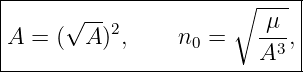
IS-GPS-200 now turns that theory into a receiver algorithm. The first part of Table 20-IV may be
organized as
The elapsed-time variable tk feeds the mean-anomaly propagation, while e, M0, Δn, and ω enter at
their appropriate points.
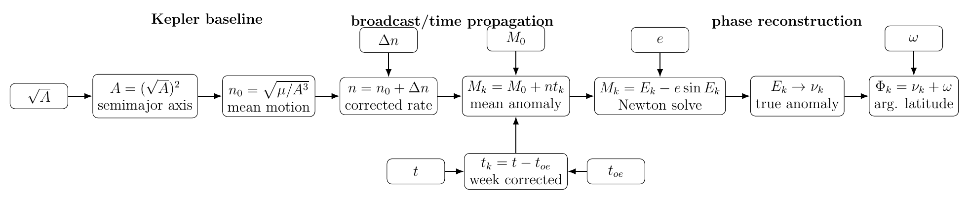
Figure 1. Computational flow from broadcast ephemeris parameters to uncorrected argument of
latitude.
The current GPS interface-document page lists IS-GPS-200N as the base revision and later
interface-revision notices. This article derives the legacy LNAV user equations appearing in Table
20-IV of Revision N; current IRNs should always be checked when implementing an operational
receiver [2, 1].
2 The constants and transmitted quantities used here
Table 20-IV begins with the GPS-user gravitational parameter
The same sheet also states the Earth rotation rate, but that quantity is not needed until the
node-longitude and Earth-fixed-coordinate equations treated later in the sequence.
The subset of broadcast quantities needed in this article is summarized below.
| Broadcast quantity | Meaning | Broadcast unit in LNAV |
 | square root of semimajor axis |  |
| Δn | mean-motion correction | semicircles/s |
| M0 | mean anomaly at reference epoch | semicircles |
| e | eccentricity | dimensionless |
| toe | ephemeris reference time | s |
| ω | argument of perigee | semicircles |
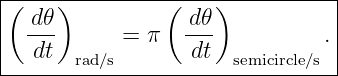
The user equations use ordinary radian trigonometric functions. Therefore a quantity transmitted
in semicircles is converted by
Likewise,
This unit conversion is essential because n0 computed from μ and A is naturally in radians per
second.
3 Step 1: recover the semimajor axis
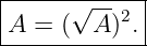
The LNAV message transmits  , not A itself. The receiver first forms
Dimensionally,
so
The result is the semimajor axis of the Keplerian-looking baseline ellipse used by the broadcast
fit.
For a GPS-like orbit,
corresponds to
The encoding also has a useful sensitivity relation. Differentiating Equation (5),
Thus the quantization of the transmitted  maps into semimajor-axis quantization through a
simple local scale factor.
maps into semimajor-axis quantization through a
simple local scale factor.
4 Step 2: derive the computed mean motion
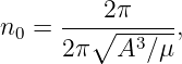
For an ideal two-body ellipse, Kepler’s third law gives
Mean motion is defined as the angular rate of mean anomaly,
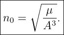
Substituting Equation (11) into Equation (12),
so
The dimensions are
Because angular measure in the user equations is radians, this is interpreted as radians per
second.
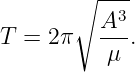
For A = 26, 560 km,
The corresponding period is
consistent with the familiar approximately twelve-hour GPS orbital period.
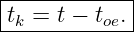
5 Step 3: form the time from ephemeris epoch
The next quantity is
Here toe is the ephemeris reference epoch and t is GPS system time associated with the signal
transmission epoch used for the satellite-position calculation. IS-GPS-200 notes that the time used
in this equation is the transmission time, meaning the reception time has effectively been corrected
for signal transit time [1].
This distinction matters. A GNSS receiver wants the satellite position when the electromagnetic
signal left the satellite, not where the satellite is when the signal arrives at the antenna.
5.1 Why a week-crossover rule is necessary
GPS seconds-of-week repeat every
A simple subtraction can therefore return a value almost one week long when the physical time
separation is only a few minutes.
IS-GPS-200 requires the actual total time difference and applies a half-week rule:
The number 302400 s is exactly one half of a GPS week.
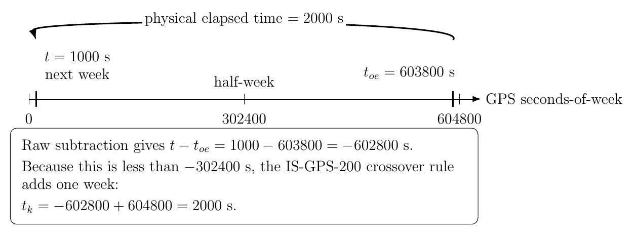
Figure 2. GPS week crossover can make a short physical interval look almost one week long unless
the half-week correction is applied.
An implementation-friendly equivalent is to map the raw difference into the interval
The conditional form in Equation (20) has the advantage of matching the interface specification
directly.
6 Step 4: apply the mean-motion correction
If the orbit were exactly Keplerian, Equation (14) would determine the phase rate completely from
A. GPSORB11 explained why the broadcast curve fit provides additional freedom through
Δn.
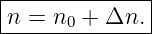
After converting Δn from semicircles per second to radians per second, the receiver
forms
The correction is therefore an additive adjustment to the Keplerian phase rate.
The distinction between n0 and n is worth preserving in software and derivations:
If Δn were accidentally added before converting semicircles/s to rad/s, the result would be wrong
by a factor of π.
7 Step 5: propagate mean anomaly
At the reference epoch,
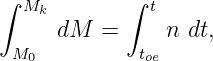
With corrected mean motion n assumed constant over this part of the broadcast model,
Integrating from toe to t,
which yields
Using tk = t − toe,
This equation is the first place where the initial orbital phase M0, the fitted phase-rate correction
Δn, and the receiver evaluation time all meet.
Mean anomaly can be normalized modulo 2π for convenience,
but the trigonometric equations themselves do not require such normalization. Keeping an
unwrapped phase can sometimes be useful for diagnostics, while a wrapped phase can improve
readability and numerical bookkeeping.
8 Step 6: solve Kepler’s equation for eccentric anomaly
Mean anomaly is linear in time, but it is not the geometric angle of the satellite on the ellipse.
GPSORB06 derived the area relation
where E is eccentric anomaly.
At time tk, the receiver therefore must solve
Because Ek appears both linearly and inside a sine function, there is no elementary algebraic
rearrangement that isolates Ek. A numerical root must be found.
8.1 Deriving the Newton-Raphson iteration
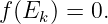
Define
The desired eccentric anomaly satisfies
Differentiate:
Newton’s method is
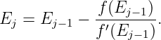
Substituting Equations (32) and (34),
Rearranging the numerator gives the form used by IS-GPS-200:
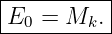
The specified initial value is
Revision N states that the refinement uses a minimum of three iterations before the final Ek is
taken from the refined value [1].
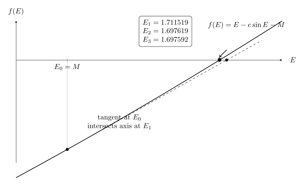
Figure 3. Newton iteration replaces the nonlinear Kepler equation by a sequence of tangent-line
root estimates.
8.2 Why the denominator is well behaved for an ellipse
For an elliptic orbit,
Because
we have
Thus the denominator in Equation (37) cannot vanish for an ordinary elliptic orbit. This is also
the same factor appearing in
so its positivity has a direct geometric meaning: orbital radius remains positive.
9 Step 7: convert eccentric anomaly to true anomaly
The receiver now knows Ek, but the orbital-plane geometry developed in GPSORB04 and
GPSORB08 is naturally expressed with true anomaly νk.
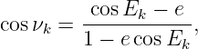
For an ellipse,
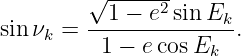
and
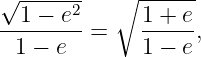
Because the common denominator is positive for e < 1, the quadrant of νk is determined by the
numerator pair. A robust implementation is therefore
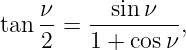
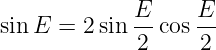
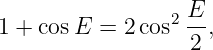
9.1 Deriving the half-angle form
Using
and substituting Equations (43)–(44),
The denominator factors as
Using
and
we obtain
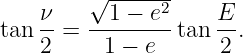
Since
then
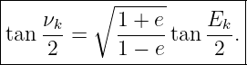
This is the relation appearing in the Table 20-IV true-anomaly equation.
For software, a particularly robust half-angle implementation is
Equation (54) and Equation (45) are equivalent. Both preserve the quadrant without having to
infer it from a single-argument inverse tangent.
10 Step 8: form the argument of latitude
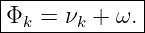
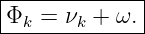
Table 20-IV sheet 2 begins with the next quantity in the chain,
This is called the argument of latitude before harmonic correction.
The geometry is simple but important:
- ω is measured in the orbital plane from the ascending-node direction to periapsis;
- νk is measured from periapsis to the satellite;
- therefore Φk is measured directly from the ascending-node direction to the satellite.
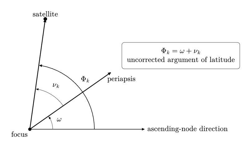
Figure 4. The uncorrected argument of latitude is the sum of argument of perigee and true
anomaly.
The notation matters because Table 20-IV next applies the twice-per-revolution corrections from
GPSORB11. Thus
is the uncorrected argument of latitude, while the later
is the corrected argument of latitude. Keeping Φk and uk as distinct variables prevents a common
implementation error.
11 A complete line-by-line numerical example
Consider the following GPS-like decoded quantities. Angular quantities are stated here directly in
radians or radians per second after any required semicircle conversion:
and choose
1. Semimajor axis
Therefore
2. Computed mean motion
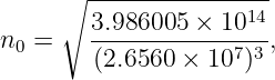
Using μ = 3.986005 × 10¹⁴ m3∕s2,
so
3. Corrected mean motion
so
4. Mean anomaly
therefore
which gives
5. Eccentric anomaly by Newton iteration
Initialize
Equation (37) gives
and
Thus after three refinements,
The second and third results already agree to the shown precision because the eccentricity is
small.
6. True anomaly
Use the quadrant-safe form
The result is
In degrees,
7. Argument of latitude
Finally,
so
This is the phase angle used by the second-harmonic correction equations in the next sheet of
Table 20-IV.
12 Sanity checks that catch common receiver bugs
The first-half algorithm is compact enough that several independent checks are inexpensive.
Dimensional check
The units should progress as
A mismatch usually indicates failure to convert a semicircle quantity to radians.
Circular-orbit limit
If
then Kepler’s equation becomes
and Equations (43)–(44) reduce to
Therefore
modulo 2π. A circular test case is therefore an excellent unit test.
Kepler residual
After solving for Ek, compute
The residual should be numerically near zero. This directly tests the iterative solver independently
of the later angle conversion.
Two true-anomaly formulas
Compute νk using both Equation (45) and Equation (54). Their wrapped angular difference
should be near machine precision. This is a strong test for quadrant mistakes.
Week-crossover test
Explicitly test epochs just before and after the GPS week boundary. The example in Figure 2
should return
not
13 Compact implementation sequence
Once the derivations are understood, the operational sequence is short:
-
1.
- Decode
 , e, toe, Δn, M0, and ω.
-
2.
- Convert all semicircle angles and angular rates to radians and radians per second.
-
3.
- Compute A = (
 )2.
)2.
-
4.
- Compute n0 =
 .
.
-
5.
- Compute tk = t − toe and apply the half-week crossover rule.
-
6.
- Compute n = n0 + Δn.
-
7.
- Compute Mk = M0 + ntk.
-
8.
- Set E0 = Mk and perform at least three Newton refinements using Equation (37).
-
9.
- Convert Ek to νk with a quadrant-safe formula.
-
10.
- Form Φk = νk + ω.
The next sheet then applies the second-harmonic corrections to Φk, radius, and inclination before
constructing the Earth-fixed satellite coordinates.
14 How this maps back to the physics
Every line of this part of Table 20-IV now has a physical origin:
| User equation | Physics or modeling origin |
| A = ( )2 )2 | Broadcast encoding of fitted orbital size |
| n0 =  | Kepler’s third law |
| tk = t − toe | Propagation from ephemeris reference epoch |
| n = n0 + Δn | Fitted correction to along-track phase rate |
| Mk = M0 + ntk | Uniform mean-anomaly propagation |
| Mk = Ek − e sin Ek | Kepler’s area law expressed through eccentric anomaly |
| Newton iteration | Numerical inversion of the nonlinear Kepler equation |
| Ek → νk | Ellipse geometry |
| Φk = νk + ω | Orbital-plane angular geometry from ascending node to
satellite |
The apparent collection of unrelated receiver formulas is therefore one continuous mechanics
chain.
15 Summary
The first half of the legacy GPS broadcast user algorithm can be compressed to
solved by Newton iteration,
and finally
The next article can continue with Table 20-IV sheet 2: δuk, δrk, δik, corrected uk, rk, ik,
orbital-plane coordinates, corrected node longitude, and the final ECEF position.
References
[1] Global Positioning Systems Directorate, IS-GPS-200N: NAVSTAR GPS Space
Segment/Navigation User Interfaces, 1 August 2022, especially Tables 20-III and 20-IV
and Section 20.3.3.4. Available from GPS.gov.
[2] GPS.gov, Interface Control Documents (ICDs) and Interface Specifications (ISs),
current public-document index, accessed September 2026.
[3] E. D. Kaplan and C. J. Hegarty, eds., Understanding GPS/GNSS: Principles and
Applications, 3rd ed., Artech House, 2017.
[4] D. A. Vallado, Fundamentals of Astrodynamics and Applications, 4th ed., Microcosm
Press, 2013.
[5] O. Montenbruck and E. Gill, Satellite Orbits: Models, Methods, and Applications,
Springer, 2000.




![√ -- 1∕2
[ A ] = m](https://images.physicslibrary.org/cache/objects/1269/make4ht/GPSBroadcastEphemerisUserEquationsKeplerPropagation8x.png)
![√ --
[( A)2] = m.](https://images.physicslibrary.org/cache/objects/1269/make4ht/GPSBroadcastEphemerisUserEquationsKeplerPropagation9x.png)




![∘ -------
[n ] = m3-∕s2= s−1.
0 m3](https://images.physicslibrary.org/cache/objects/1269/make4ht/GPSBroadcastEphemerisUserEquationsKeplerPropagation18x.png)