1 The question left by the six-element orbit
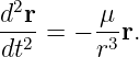
GPSORB02 established that the state of a point-mass satellite in a two-body gravitational field
has six independent degrees of freedom. GPSORB05 then expressed the same information with the
classical orbital elements
or, more conveniently for time propagation,
If six quantities determine the ideal orbit, why does a GPS LNAV ephemeris transmit additional
terms such as
and six more coefficients
The answer is that the real GPS satellite does not obey the exact two-body model over the
broadcast fit interval. The broadcast ephemeris is therefore not simply a different notation for six
exact constants of motion. It is a compact approximation to a more complicated propagated
trajectory.
The GPS interface specification makes this distinction explicit: the ephemeris parameters are
Keplerian in appearance, but the operational values are obtained by a least-squares curve fit of a
propagated satellite trajectory represented by time-position samples in Earth-fixed coordinates
[1].
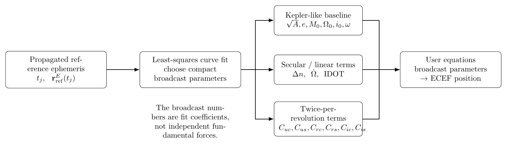
Figure 1. The GPS broadcast ephemeris is a compact fitted model of a propagated reference
trajectory.
This viewpoint is the organizing idea for the entire article.
2 A useful mathematical model of the curve fit
Suppose the control segment has a high-fidelity reference trajectory sampled at times
tj,
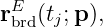
Let the broadcast model generate an Earth-fixed position
where p is the vector of broadcast ephemeris parameters.
A simplified weighted least-squares objective is
The actual GPS control-segment process is more detailed, but Equation (7) captures the essential
mathematics: choose a small set of coefficients so that a simple user algorithm reproduces the
reference trajectory closely over a finite interval.
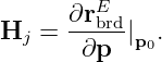
Linearizing about a trial parameter vector p0 gives
where
Stacking all observations gives the familiar least-squares update
This is important conceptually. A coefficient such as Crc is not required to equal one closed-form
force coefficient. It is a fitted amplitude that helps the user equations track the reference
orbit.
3 The broadcast model as a basis expansion
A convenient way to understand the extra parameters is to view the broadcast orbit as a truncated
basis expansion. Three kinds of basis functions are used:
-
1.
- constant terms, which set the orbit at the reference epoch;
-
2.
- linear functions of time, which represent slow drift over the fit interval;
-
3.
- sinusoidal functions of orbital phase, which represent short-period residuals.
Schematically,
where q can stand for an orbital angle, radius-like quantity, or inclination-like quantity.
Equation (11) is not one of the GPS user equations. It is a conceptual model that explains the
architecture of the broadcast parameter set.
4 Why transmit a mean-motion correction Delta-n?
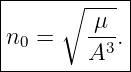
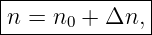
For a perfect Kepler ellipse,
and the mean motion is not independent of semimajor axis:
The mean anomaly then advances as
A real perturbed trajectory does not have to satisfy the exact two-body coupling between the
best-fit radial scale and the best-fit along-track phase rate. GPS therefore introduces one
additional degree of freedom,
so that
The physical meaning is easiest to see by defining a phase residual
Over a short fit interval, Taylor expansion gives
The fitted M0 absorbs the constant part, while Δn supplies the leading linear phase-rate
correction,
in this local approximation.
This also explains why simply adjusting A is not equivalent. Changing A affects the geometric size
of the orbit and, through Equation (13), changes the Keplerian phase rate simultaneously. The
extra Δn parameter partially decouples those two fit requirements.
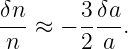
For scale intuition, differentiating n ∝ a−3∕2 gives
Equation (20) is useful sensitivity physics, but the transmitted Δn should not be interpreted
literally as a semimajor-axis error. It is a fitted mean-motion difference.
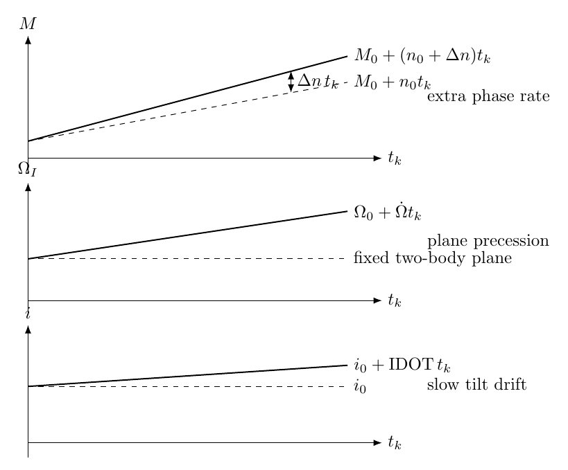
Figure 2. The three broadcast rate terms provide linear-in-time freedom in phase, node
orientation, and inclination.
4.1 Illustrative phase sensitivity
For a GPS-like semimajor axis
Equation (13) gives approximately
Consider an illustrative, not satellite-specific, correction
After two hours,
A rough along-track scale is
Thus an apparently tiny angular-rate correction can matter at navigation accuracy
scales.
5 Why transmit a node rate?
In ideal two-body motion the orbital plane is fixed, so
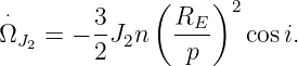
GPSORB10 showed that Earth’s oblateness breaks this result. The dominant first-order secular J2
contribution is
For a prograde GPS-like orbit this is negative, producing nodal regression.
The legacy broadcast ephemeris therefore allows the node orientation to evolve linearly. In the
GPS user equations the Earth-fixed node angle is
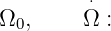
As derived in GPSORB09, the  e terms account for Earth rotation. The transmitted
  supplies
the fitted orbital-plane rate before that Earth-rotation subtraction.
supplies
the fitted orbital-plane rate before that Earth-rotation subtraction.
The J2 expression in Equation (27) explains the dominant physics, but the broadcast  is not
defined as “the J2 rate.” It is one coefficient of the curve fit to the propagated reference
ephemeris.
is not
defined as “the J2 rate.” It is one coefficient of the curve fit to the propagated reference
ephemeris.
6 Why transmit IDOT?
The GPS quantity IDOT is the rate of inclination angle. The user algorithm forms
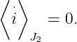
This parameter is particularly instructive. In the first-order orbit-averaged J2 model developed in
GPSORB10,
So IDOT should not be explained as merely “the J2 inclination rate.”
Real GPS orbit propagation contains additional effects: higher-degree and order gravity terms,
lunisolar gravity, solar-radiation pressure, and other modeled or empirical accelerations. Even when
a particular perturbation has zero first-order secular inclination rate, a finite-interval least-squares
approximation can benefit from a small linear inclination term. IDOT supplies that
freedom.
Thus the pair
plays the same mathematical role as
one parameter sets the orientation at the reference epoch; the other allows a slow linear
drift.
7 Why does the periodic correction use twice the orbital phase?
The six harmonic coefficients are one of the least intuitive parts of the legacy broadcast ephemeris.
Their structure becomes much less mysterious after GPSORB10.
For the J2 disturbing function,
where
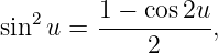
is the argument of latitude. Using
we obtain the structure
The ellipsis reminds us that the full short-period element variations also contain radial dependence
and eccentricity-dependent terms. Equation (36) nevertheless identifies the key symmetry: a
degree-two equatorially symmetric disturbance naturally creates a twice-per-revolution
signature.
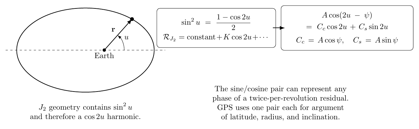
Figure 3. Degree-two gravity motivates a twice-per-revolution basis, and a sine/cosine pair
permits arbitrary phase.
8 Why both sine and cosine coefficients?
A single cosine would assume that the residual peaks at a specific reference phase. A general
second harmonic has an arbitrary phase shift,
Expanding,
Defining
gives
Thus two coefficients are exactly what is required to represent an arbitrary amplitude and phase at
harmonic number two.
Conversely,
This is why GPS carries coefficient pairs rather than a single number for each correction
channel.
9 Fourier-series interpretation of the six C coefficients
Suppose a short-period residual in some orbital quantity q is periodic in argument of latitude. It
can be represented formally by a Fourier series,
A very compact model can retain only the dominant second harmonic,
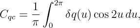
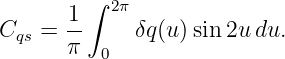
For an ideal continuously and uniformly weighted fit over a full cycle, the Fourier coefficients would
be
The actual GPS fitting process is not this simple Fourier integral, because the fitted
quantity is ultimately satellite position over a finite interval and all parameters interact.
But the projection equations show why the C values can be understood as harmonic
amplitudes.
10 The three harmonic correction channels
The user algorithm first computes the uncorrected argument of latitude
It then forms three independent second-harmonic corrections.
10.1 Argument-of-latitude correction
The corrected argument of latitude is
Because u is an in-plane angle, this correction primarily adjusts the along-track angular
geometry.
10.2 Radius correction
The corrected radius is
Here Crc and Crs have units of length.
10.3 Inclination correction
The corrected inclination is Equation (29),
This channel changes the orientation of the orbital plane and therefore contributes mainly to
cross-track position.
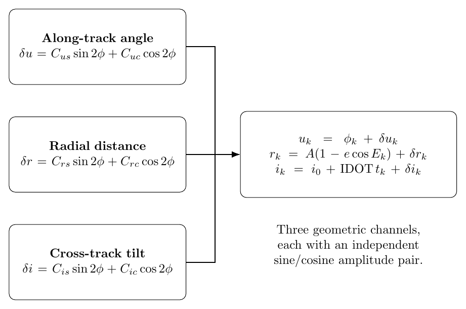
Figure 4. GPS applies independent second-harmonic corrections to along-track angle, radius, and
inclination.
11 Why these particular three channels?
A small position error near a reference orbit can be decomposed approximately into radial,
along-track, and cross-track components,
For small plane-angle errors, the cross-track scale is of order
The GPS correction structure therefore has a direct geometric interpretation:
| Correction | Geometric effect | Coefficient units |
| δu | along-track angular displacement | radians |
| δr | radial displacement | meters |
| δi | cross-track plane tilt | radians |
This does not imply a perfect one-to-one separation in the final ECEF coordinates. The rotation
from orbital coordinates couples all three channels. It does explain why these are efficient
quantities to correct.
12 Illustrative harmonic correction calculation
Consider an illustrative argument of latitude
with synthetic coefficients
These values are chosen only to illustrate the equations; they are not a broadcast record for a
particular satellite.
Since
Equation (48) gives
At a GPS-like orbital radius, the corresponding angular displacement has an along-track scale of
roughly
The radial correction is
and the inclination correction is
Again, the purpose is scale intuition: tiny angular coefficients can correspond to tens of meters at
medium-Earth-orbit radius.
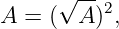
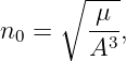
13 The complete legacy LNAV position chain
The extra parameters now fit naturally into the user algorithm. Starting with
compute the Keplerian mean motion
and then the fitted mean motion
With
propagate mean anomaly,
Solve Kepler’s equation,
and convert Ek to true anomaly νk. Form
Apply Equations (48), (50), and (52), then compute
The corrected longitude of ascending node is Equation (28). Finally,
followed by
This is the compact model Kaplan presents in algorithmic form. The previous articles in this series
now explain the physics behind every layer of it.
14 Parameter definitions in the GPS interface specification
For the legacy LNAV ephemeris, IS-GPS-200 defines the extra quantities as shown below
[1].
| Parameter | Role | Units |
| Δn | mean motion difference from computed value | angle/time |
| 
| rate of right ascension | angle/time |
| IDOT | rate of inclination angle | angle/time |
| Cuc,Cus | cosine/sine harmonic corrections to argument of
latitude | radians |
| Crc,Crs | cosine/sine harmonic corrections to orbital radius | meters |
| Cic,Cis | cosine/sine harmonic corrections to inclination | radians |
The specification also defines the broadcast parameters as outputs of a curve fit to a
propagated orbit rather than as direct measurements of isolated physical perturbations
[1].
15 What the coefficients do not mean
Several tempting interpretations should be avoided.
-
1.
- Δn is not simply “the effect of J2 on mean motion.” It is a fitted correction to the
Keplerian mean-motion relation.
-
2.
 is strongly motivated by J2 nodal regression, but the broadcast value is a fitted orbit
parameter, not a pure analytic J2 coefficient.
is strongly motivated by J2 nodal regression, but the broadcast value is a fitted orbit
parameter, not a pure analytic J2 coefficient.
-
3.
- IDOT is not the first-order secular J2 inclination rate; that secular rate is zero in the
simple averaged model.
-
4.
- Cuc through Cis are not six fundamental gravity coefficients. They are amplitudes in
the chosen broadcast correction basis.
-
5.
- The presence of more than six broadcast numbers does not imply that the satellite
has more than six instantaneous Cartesian state variables. The additional numbers
describe how a compact approximate model reproduces a perturbed trajectory over
time.
16 Why no explicit omega-dot in legacy LNAV?
GPSORB10 showed that J2 produces secular apsidal precession,
Yet the legacy LNAV parameter set does not transmit a separate  term.
term.
This is another reminder that the broadcast model is an engineered approximation basis, not a list
containing one coefficient for every physical secular rate. Over the relatively short fit interval, the
effects associated with periapsis motion can be absorbed among the fitted ω, M0, Δn,
eccentricity, and harmonic corrections well enough to meet the broadcast-orbit accuracy
objective.
A different navigation-message design can choose a different basis. The modernized CNAV
formulation, for example, includes additional parameters such as a semimajor-axis rate and a
mean-motion-difference rate [1]. That evolution reinforces the main point: the parameterization is
chosen for compact approximation performance.
17 A hierarchy of models
It is useful to keep four levels separate:
-
1.
- Two-body dynamics:
Six constants describe the exact solution.
-
2.
- Analytic perturbation theory: add forces such as J2 and derive secular and periodic
element changes.
-
3.
- High-fidelity orbit propagation: numerically propagate a detailed force model and
estimation solution.
-
4.
- Broadcast ephemeris: fit a compact, standardized parameter set so a receiver can
reconstruct satellite position efficiently.
Confusing these levels is the main source of difficulty when first reading the GPS ephemeris
equations.
18 Connection to Kaplan’s table
Kaplan’s sequence becomes conceptually transparent when grouped by model layer:
| Layer | Equations |
| Kepler baseline | A, n0, Mk, Ek, νk |
| Fitted secular corrections | n = n0 + Δn, i0 + IDOT tk, Ωk with  |
| Fitted periodic
corrections | δuk, δrk, δik from the six C coefficients |
| Geometry | uk, rk, ik, then orbital-plane x′k,y′k |
| Earth-fixed coordinates | final xk,yk,zk rotation using Ωk |
Thus the “extra” parameters are exactly the bridge between ideal celestial mechanics and a
receiver-friendly representation of the real orbit.
19 Summary
The legacy GPS ephemeris can be understood as
The roles are:
The degree-two symmetry of J2 explains why twice-per-revolution structure is physically natural,
but the transmitted coefficients themselves are best understood as fitted parameters of the
standardized broadcast model.
The next article, GPSORB12, can now derive the first half of the IS-GPS-200 user algorithm line
by line: A, n0, corrected n, tk, Mk, the iterative solution of Kepler’s equation, true anomaly, and
the argument of latitude.
References
[1] Global Positioning Systems Directorate, IS-GPS-200N: NAVSTAR GPS Space
Segment/Navigation User Interfaces, 1 August 2022, especially Tables 20-II, 20-III, and
20-IV and Sections 20.3.3.4.2–20.3.3.4.3. Available from GPS.gov and the U.S. Coast
Guard Navigation Center.
[2] E. D. Kaplan and C. J. Hegarty, eds., Understanding GPS/GNSS: Principles and
Applications, 3rd ed., Artech House, 2017.
[3] D. A. Vallado, Fundamentals of Astrodynamics and Applications, 4th ed., Microcosm
Press, 2013.
[4] O. Montenbruck and E. Gill, Satellite Orbits: Models, Methods, and Applications,
Springer, 2000.
[5] W. M. Kaula, Theory of Satellite Geodesy, Blaisdell Publishing, 1966.






![N
∑ [ E E ]T [ E E ]
J (p ) = rref(tj) − rbrd(tj;p) Wj r ref(tj) − rbrd(tj;p) .
j=1](https://images.physicslibrary.org/cache/objects/1267/make4ht/GPSBroadcastsExtraEphemerisParametersDeltaNNodeAndInclinationRatesAndHarmonicCorrections6x.png)






![δM (t) = Mref (t) − [M0 + n0tk].](https://images.physicslibrary.org/cache/objects/1267/make4ht/GPSBroadcastsExtraEphemerisParametersDeltaNNodeAndInclinationRatesAndHarmonicCorrections16x.png)




















![∞
∑
δq(u) = a0 + [am cos(mu ) + bm sin(mu )].
m=1](https://images.physicslibrary.org/cache/objects/1267/make4ht/GPSBroadcastsExtraEphemerisParametersDeltaNNodeAndInclinationRatesAndHarmonicCorrections45x.png)