1 Why the two-body ellipse is not quite enough
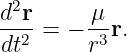
GPSORB01–GPSORB09 developed the ideal Kepler problem from
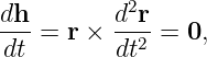
Because the force is central,
so the orbital plane is fixed. The eccentricity vector is also constant, so periapsis is fixed within
that plane.
Real Earth violates the spherical assumption. Its equatorial radius is larger than its polar radius,
and the external gravity field is therefore not exactly proportional to 1∕r. The largest correction is
the degree-two zonal harmonic J2.
The immediate consequences are important:
-
1.
- the acceleration is no longer exactly parallel to −r;
-
2.
- the specific angular momentum vector can slowly change direction;
-
3.
- the ascending node can regress or advance;
-
4.
- the periapsis direction can precess within the orbital plane.
These effects are small during one revolution, but they accumulate over many orbits. That makes
them especially important for a long-lived navigation Constellation.
2 External gravity as a multipole expansion
Outside Earth’s mass distribution the gravitational potential satisfies Laplace’s equation,
For an axisymmetric body, there is no longitude dependence. Separation of variables in spherical
coordinates gives an exterior solution of the form
Here 𝜃 is geocentric colatitude, RE is a reference equatorial radius, Pℓ is a Legendre polynomial,
and Jℓ is a dimensionless zonal coefficient.
The monopole term ℓ = 0 is the familiar spherical potential −μ∕r. The dipole term ℓ = 1 vanishes
when the origin is placed at Earth’s center of mass. The leading departure from sphericity is
therefore the quadrupole term ℓ = 2.
Using geocentric latitude ϕ = π∕2 − 𝜃 gives
and
Keeping only J2 in Equation (4),
Equivalently,
The second term is the J2 perturbing potential per unit mass.
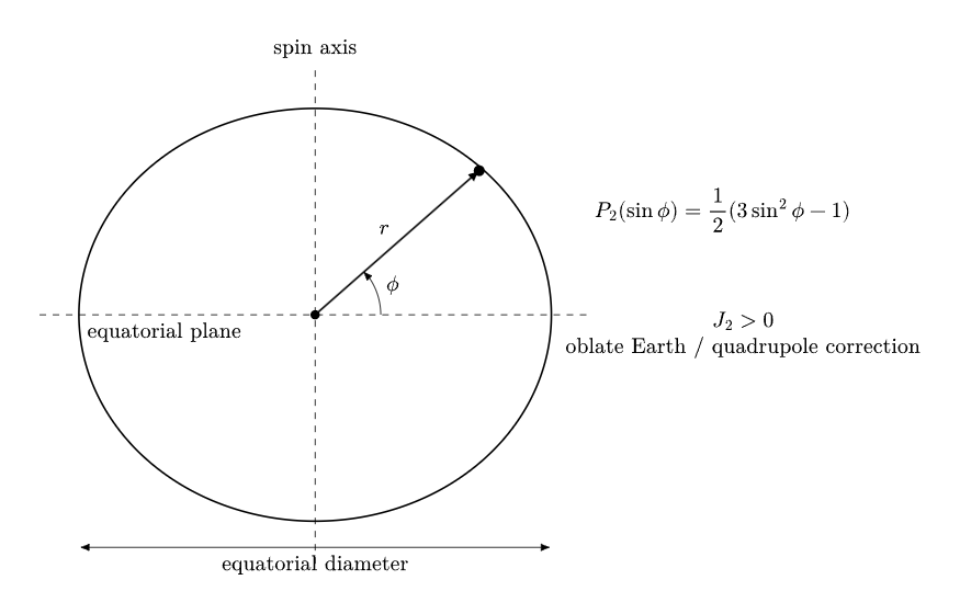
Figure 1. Geometry of the leading degree-two zonal correction to Earth’s gravity field.
For Earth, J2 is positive and approximately
The small number is deceptive: a part-per-thousand distortion of the dominant gravity field is
easily large enough to rotate orbital orientation by many degrees over a year.
3 From potential to the J2 acceleration
The acceleration follows from
Writing
Equation (8) can be differentiated in Cartesian coordinates. The total acceleration through degree
two is
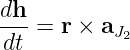
The correction is not generally parallel to r. Therefore
is generally nonzero. This is the physical origin of orbital-plane precession.
4 Geometry inside the orbital plane
Let
be the argument of latitude, where ω is the argument of periapsis and ν is true anomaly. For an
orbit inclined by i to the equator, the geocentric latitude satisfies
This relation is the key bridge between the Earth-fixed symmetry of J2 and the satellite’s orbital
elements.
Substituting Equation (17) into the perturbing potential gives
It is convenient in the Lagrange planetary equations to define the disturbing function as the
negative perturbing potential,
Hence
Equation (20) contains both short-period terms and terms that survive orbital averaging. The
secular changes come from the orbit-averaged disturbing function.
5 Averaging the J2 disturbing function
For a Keplerian reference ellipse,
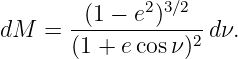
The relation between mean anomaly and true anomaly is
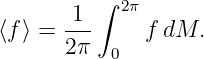
An average over one orbital period is therefore
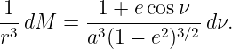
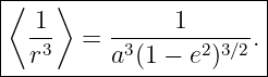
First evaluate ⟨r−3⟩. Using the equations above,
Integrating from 0 to 2π removes the cosine term, giving
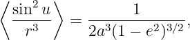
Next,
because the average of sin 2(ω + ν) is 1∕2, while the additional term proportional to e cos ν
integrates to zero over a full revolution.
Applying Equations (25) and (26) to Equation (20),
This single averaged scalar function contains the first-order secular J2 rates.
6 Lagrange planetary equation for the ascending node
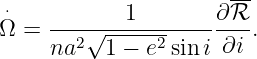
For an averaged disturbing function that is independent of the node itself, the Lagrange planetary
equation for Ω is
Differentiate Equation (27):
Substitute into Equation (28):
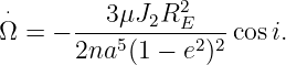
Using
and
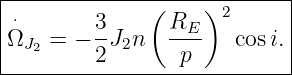
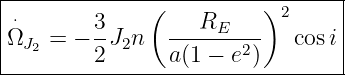
we obtain the standard secular nodal rate
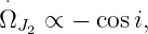
For a prograde orbit with 0 < i < 90∘, cos i > 0, so
The ascending node regresses.
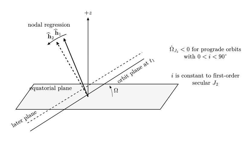
Figure 2. The J2 torque causes the orbit normal and ascending node to precess about Earth’s
symmetry axis.
For a polar orbit, i = 90∘ and the first-order secular node rate vanishes. For a retrograde orbit,
cos i < 0 and the sign reverses.
7 Lagrange planetary equation for periapsis
The argument of periapsis is affected both by the eccentricity dependence of the disturbing
function and by the moving node. With the present disturbing-function convention,
Differentiate Equation (27) with respect to eccentricity. Since
we obtain
The first term in Equation (35) becomes
The node-coupling term is
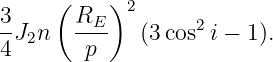
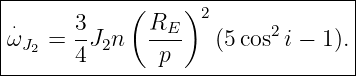
Adding the two pieces gives
This is apsidal precession: the eccentricity vector rotates inside the orbital plane.
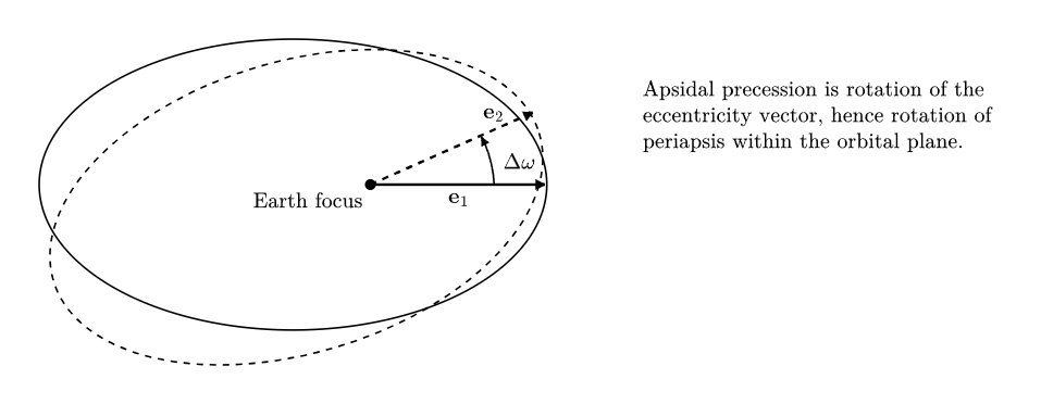
Figure 3. Apsidal precession rotates the eccentricity vector and periapsis direction within the
orbital plane.
8 The critical inclination
Equation (40) vanishes when
Therefore
and
These are the classical critical inclinations. At this first-order J2 level, the argument of periapsis
has no secular drift there.
GPS uses an inclination near 55∘, not the critical inclination, so both nodal and apsidal secular
effects are present.
9 What remains constant in the first-order secular J2 model
The averaged J2 model has an important structure. To first order in the secular approximation,
But
Thus the orbit keeps approximately the same size, shape, and inclination while its orientation
changes.
This does not mean the instantaneous elements are perfectly constant. The unaveraged J2
acceleration produces short-period variations in several elements. The statements above refer only
to the leading first-order secular behavior.
There is also a useful symmetry interpretation. Because the J2 potential is axisymmetric about
Earth’s spin axis, the potential does not depend on inertial longitude. The component of angular
momentum along the symmetry axis is therefore conserved. The full angular-momentum vector can
precess while maintaining its projection on z.
10 Inclination dependence of the two secular rates
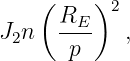
Both secular rates scale with
but their inclination dependence differs:
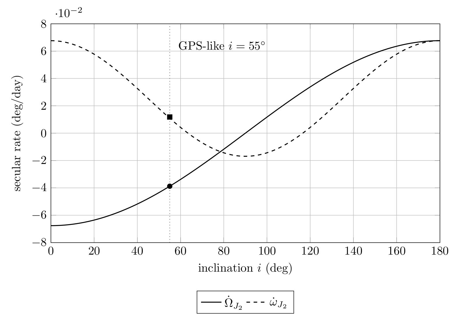
Figure 4. First-order J2 secular rates versus inclination for a GPS-like medium-Earth orbit.
The node rate changes sign at 90∘. The apsidal rate changes sign at the two critical
inclinations.
11 Numerical example for a GPS-like orbit
Use representative values
with
and
The semilatus rectum is
The Keplerian mean motion is
corresponding to an orbital period of approximately
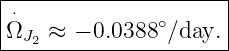
Substituting into Equation (33),
Over one year, the pure first-order J2 contribution would accumulate to roughly
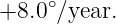
For periapsis,
or about
Across a two-hour interval, however, these changes are only about
The rates are small over one broadcast-ephemeris interval but large over the lifetime of a
satellite.
12 Connection to GPS constellation behavior
The GPS space segment uses medium-Earth orbits with nominal inclination near 55∘. The
GPS Standard Positioning Service Performance Standard lists a 55 degree reference
inclination, and official constellation descriptions place the satellites near 20,200 km
altitude.
The J2 nodal-regression estimate above is therefore physically representative of GPS. It explains
why an inertial ascending node cannot be treated as a permanent constant over months or
years.
It is important, however, to distinguish three different quantities:
-
1.
- the ideal two-body constant Ω;
-
2.
- the analytic first-order perturbation rate
 J2;
J2;
-
3.
- the broadcast ephemeris coefficient
 transmitted by GPS.
The third is not merely Equation (33) copied into the navigation message. The broadcast
ephemeris parameters are fitted so that the user equations reproduce a high-fidelity propagated
trajectory over a limited fit interval. The fitted rate therefore represents the behavior
required by that broadcast model, including more physics than the single analytic J2
term.
13 Why the legacy broadcast model contains a node rate but not an explicit periapsis
rate
The legacy GPS ephemeris includes parameters such as
as well as six harmonic correction coefficients. The user algorithm explicitly propagates the node
longitude with a rate and propagates inclination with IDOT.
The legacy model does not transmit a separate  term. This does not imply that real periapsis is
physically stationary. Rather, ω is part of a short-arc fitted ephemeris, and residual orbital
behavior is represented by the fitted element set and harmonic corrections over the applicable
interval.
term. This does not imply that real periapsis is
physically stationary. Rather, ω is part of a short-arc fitted ephemeris, and residual orbital
behavior is represented by the fitted element set and harmonic corrections over the applicable
interval.
This distinction matters for learning the physics: Equation (40) tells us why periapsis should
precess in a real oblate gravity field, even though the legacy broadcast parameterization chooses
not to expose that physical rate as a separate user parameter.
14 Why J2 also hints at the harmonic correction structure
Equation (20) contains
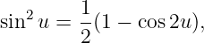
Using
we immediately see why degree-two gravity naturally produces second-harmonic structure
involving
and, after the full perturbation solution is developed,
This is the physical clue behind the GPS correction form
with analogous radius and inclination corrections.
The broadcast coefficients should not be identified one-for-one with a single closed-form J2
perturbation coefficient. They are fitted parameters. But the double-angle structure is exactly what
one expects when the leading nonspherical gravity term is degree two.
15 Beyond J2
A realistic GPS orbit model contains additional perturbations,
Higher geopotential harmonics, third-body gravitation, solar radiation pressure, Earth radiation
effects, and maneuver history all contribute to the precise trajectory.
The purpose of J2 is not to replace that high-fidelity model. Its value is that it is the
first perturbation for which the ideal Kepler picture visibly breaks in a systematic,
derivable way. It explains two of the most important qualitative facts about real satellite
orbits:
and
16 Summary
The main derivation chain is
followed by
The two key secular rates are
and
For a GPS-like orbit near 55∘ inclination, the first is negative and the second is positive. These
rates supply the physical bridge from the fixed Keplerian orientation of GPSORB05–GPSORB09
to the slowly changing orbital geometry represented by real GPS ephemerides.
References
[1] E. D. Kaplan and C. J. Hegarty, eds., Understanding GPS/GNSS: Principles and
Applications, 3rd ed., Artech House, 2017.
[2] D. A. Vallado, Fundamentals of Astrodynamics and Applications, 4th ed., Microcosm
Press, 2013.
[3] O. Montenbruck and E. Gill, Satellite Orbits: Models, Methods and Applications,
Springer, 2000.
[4] H. D. Curtis, Orbital Mechanics for Engineering Students, 4th ed., Elsevier, 2020.
[5] U.S. Space Force, IS-GPS-200N: Navstar GPS Space Segment/Navigation User
Interfaces, 1 August 2022.
[6] U.S. Government, Global Positioning System Standard Positioning Service
Performance Standard, 5th ed., April 2020.
[7] National Geospatial-Intelligence Agency, World Geodetic System 1984 (WGS 84),
Office of Geomatics.


![[ ∞∑ ( ) ℓ ]
V (r,𝜃 ) = − μ 1 − J RE-- P (cos𝜃) .
r ℓ r ℓ
ℓ=2](https://images.physicslibrary.org/cache/objects/1266/make4ht/J2GravityPerturbationNodalRegressionAndApsidalPrecessionForGPSOrbits3x.png)


![[ ]
μ ( R )2 1
V(r,ϕ) = − -- 1 − J2 --E- --(3sin2ϕ − 1) .
r r 2](https://images.physicslibrary.org/cache/objects/1266/make4ht/J2GravityPerturbationNodalRegressionAndApsidalPrecessionForGPSOrbits6x.png)




![[ ( ) ( ) ]
μx 3 RE 2 z2
ax = − --3 1 + -J2 ---- 1 − 5-2- ,
r 2 r r](https://images.physicslibrary.org/cache/objects/1266/make4ht/J2GravityPerturbationNodalRegressionAndApsidalPrecessionForGPSOrbits11x.png)
![[ ( ) ( ) ]
μy 3 RE 2 z2
ay = − -r3 1 + 2J2 -r-- 1 − 5 r2 ,](https://images.physicslibrary.org/cache/objects/1266/make4ht/J2GravityPerturbationNodalRegressionAndApsidalPrecessionForGPSOrbits12x.png)
![[ ( ) ( ) ]
μz- 3- RE-- 2 z2-
az = − r3 1 + 2J2 r 3 − 5 r2 .](https://images.physicslibrary.org/cache/objects/1266/make4ht/J2GravityPerturbationNodalRegressionAndApsidalPrecessionForGPSOrbits13x.png)