1 Where GPSORB13 begins
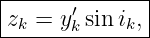
GPSORB12 derived the first half of the legacy broadcast-position algorithm:
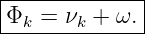
with
The quantity Φk is the uncorrected argument of latitude: the angle in the orbital plane from the
ascending-node direction to the satellite before the broadcast second-harmonic corrections are
applied.
The second sheet of IS-GPS-200 Table 20-IV continues with the sequence
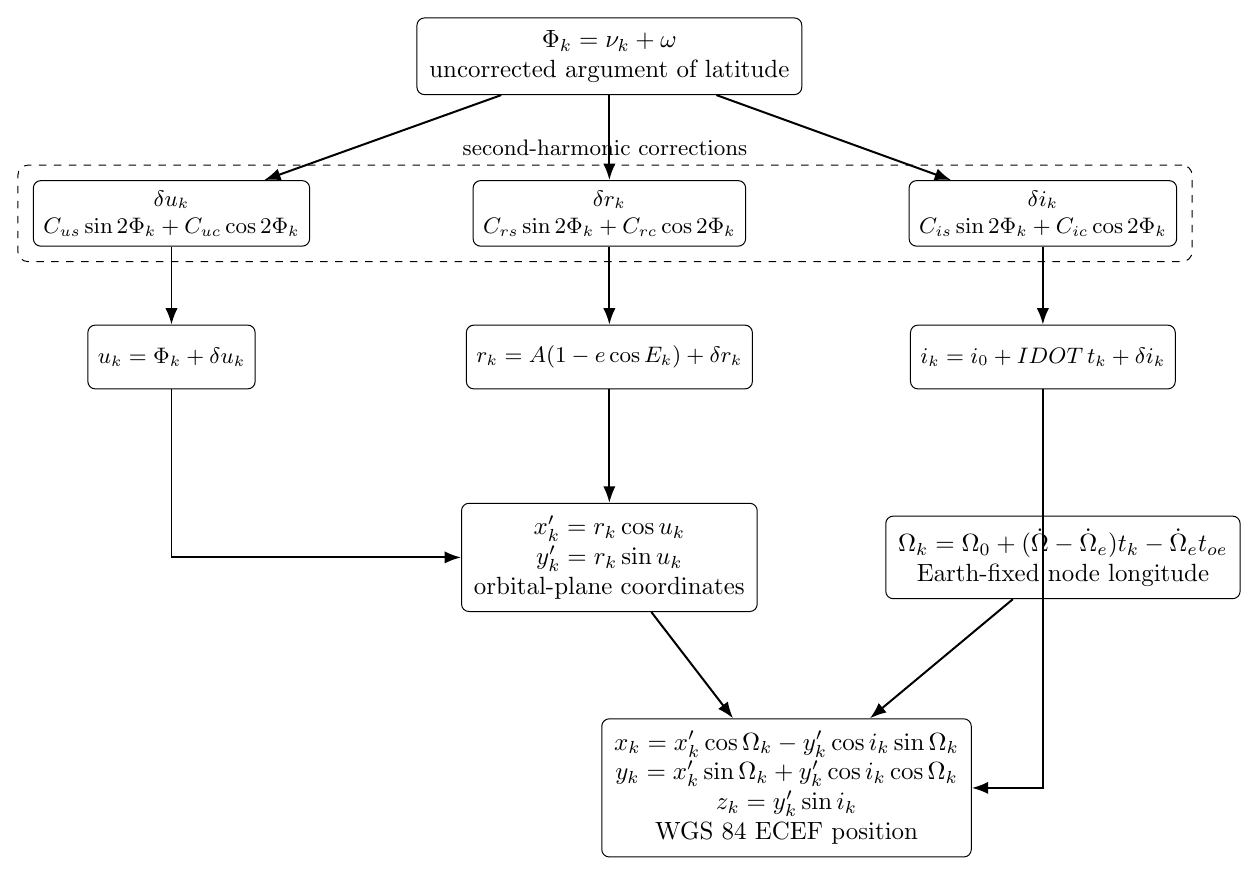
Figure 1. Computational flow through the second sheet of the legacy GPS broadcast position
algorithm.
The current GPS public-document index identifies IS-GPS-200N as the current base revision of the
L1/L2 space-to-user interface specification. This article derives the legacy LNAV Table 20-IV
equations in Revision N; an operational implementation should also check any applicable
interface-revision notices [2, 1].
2 Broadcast quantities used in this half of the calculation
In addition to A, e, Ek, Φk, tk, and toe already available from GPSORB12, the second-half position
calculation uses
| Broadcast quantity | Meaning | LNAV units |
| Cuc | cosine correction to argument of latitude | radians |
| Cus | sine correction to argument of latitude | radians |
| Crc | cosine correction to orbital radius | meters |
| Crs | sine correction to orbital radius | meters |
| Cic | cosine correction to inclination | radians |
| Cis | sine correction to inclination | radians |
| i0 | inclination at reference epoch | semicircles |
| IDOT | inclination-rate correction | semicircles/s |
| Ω0 | longitude of ascending-node plane at weekly epoch | semicircles |
| node-rate parameter | rate of right ascension | semicircles/s |
IS-GPS-200 denotes the node-rate parameter by  . Table 20-III gives the harmonic latitude and
inclination coefficients directly in radians, while the radial pair is in meters. The node,
inclination, and rate parameters transmitted in semicircles or semicircles per second must be
converted to radians or radians per second before being mixed with radian-valued quantities
[1].
. Table 20-III gives the harmonic latitude and
inclination coefficients directly in radians, while the radial pair is in meters. The node,
inclination, and rate parameters transmitted in semicircles or semicircles per second must be
converted to radians or radians per second before being mixed with radian-valued quantities
[1].
The GPS user value of the Earth rotation rate is
3 Step 1: why the correction functions use twice the argument of latitude
GPSORB10 showed that the leading nonspherical Earth-gravity perturbation contains degree-two
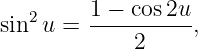
angular structure. In orbital geometry one encounters terms such as
Using
reveals a natural twice-per-revolution harmonic. GPSORB11 then emphasized an important
modeling distinction: the broadcast coefficients are not obtained by simply substituting a
closed-form J2 solution. They are fitted coefficients in the prescribed broadcast model, but a
sine/cosine basis at 2Φk is physically well matched to the dominant degree-two periodic
structure.
Over one full revolution of Φ, both sin 2Φ and cos 2Φ complete two cycles.
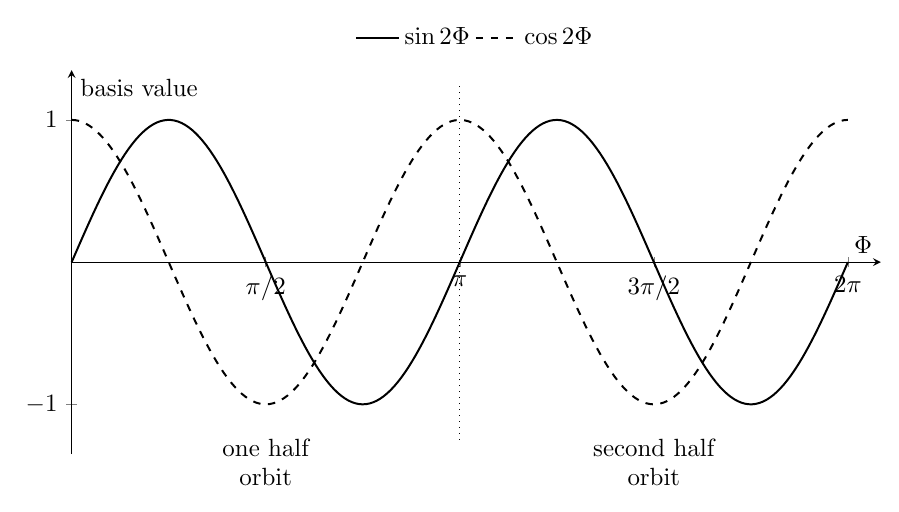
Figure 2. The two basis functions used by the broadcast harmonic corrections repeat twice per
orbital revolution.
A general second harmonic with arbitrary phase can be written
Therefore a pair of coefficients multiplying sine and cosine can represent both amplitude and
phase. If
then
This is why each corrected orbital quantity receives a pair of harmonic coefficients rather than a
single amplitude.
4 Step 2: argument-of-latitude correction
The first Table 20-IV correction is
Both coefficients have angular units, so
The receiver then applies the correction directly to the uncorrected argument of latitude:
The notation is worth preserving carefully:
while
A software implementation that overwrites Φk too early can obscure which angle belongs in the
harmonic terms.
5 Step 3: radial correction
The corresponding radial harmonic is
Because Crs and Crc are measured in meters,
Before this correction is added, the Keplerian ellipse geometry from GPSORB06 gives
That result follows directly from the focus-centered eccentric-anomaly parameterization of the
ellipse.
The GPS broadcast model modifies the radius by
It is useful to read Equation (18) as
6 Step 4: inclination correction and IDOT
The harmonic inclination correction is
Again,
The complete corrected inclination is
This equation contains three distinct pieces:
and
As emphasized in GPSORB11, IDOT should not be interpreted as a claim that first-order secular
J2 theory predicts a nonzero mean inclination rate. The broadcast value is a fitted coefficient for
the complete propagated reference trajectory.
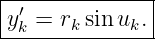
7 Step 5: form the corrected orbital-plane coordinates
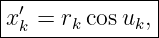
After uk and rk are known, the satellite’s coordinates in the corrected orbital plane are ordinary
polar-to-Cartesian relations:
The x′k direction lies along the ascending-node direction in the orbital plane, and the y′k axis is
90∘ ahead within that plane.
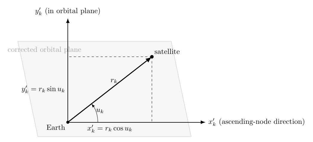
Figure 3. Corrected radius and argument of latitude resolve the satellite position into
node-aligned orbital-plane coordinates.
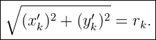
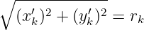
The equations immediately provide a useful invariant:
so
This is an inexpensive software sanity check.
8 Step 6: corrected longitude of the ascending node
GPSORB09 derived the Earth-fixed node equation from the difference between inertial node
motion and Earth rotation. Table 20-IV uses
Because
Equation (30) may be rearranged as
This alternate form exposes the physics:
 (t − toe) propagates the fitted orbital-node orientation;
- −
 et accounts for the rotation of the Earth-fixed axes beneath the orbit.
A common implementation concern is the size of Ωk. Trigonometric functions are periodic, so it is
mathematically acceptable to use the unwrapped value. In numerical software it is often convenient
to reduce it modulo 2π before evaluating sines and cosines.
9 Step 7: derive the final ECEF rotation
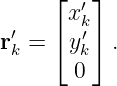
The orbital-plane vector is
The geometry is the same rotation structure derived in GPSORB08, but the quantities are now the
corrected broadcast quantities and Ωk is already an Earth-fixed node longitude.
First tilt the orbital plane by the corrected inclination ik, then rotate the node direction by Ωk.
With the rotation convention used throughout this series,
The combined matrix is
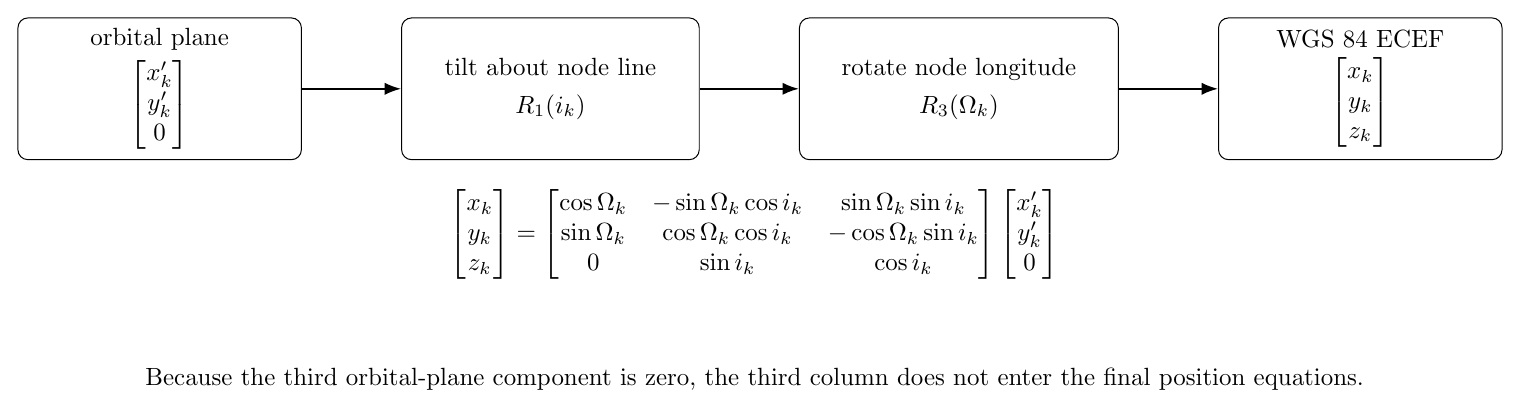
Figure 4. The corrected orbital-plane coordinates are tilted by inclination and rotated by the
Earth-fixed node longitude.
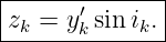
Because the third component of r′k is zero, Equation (35) reduces immediately to the three Table
20-IV equations:
IS-GPS-200 identifies these as the satellite antenna phase-center coordinates in the WGS 84
Earth-centered Earth-fixed coordinate system [1].
10 Why there is no extra ECI-to-ECEF rotation afterward
This point deserves emphasis because it is an easy place to double-count Earth rotation.
In a conventional inertial orbital-elements calculation one might first form an inertial position
vector
after which a separate Earth-rotation matrix converts ECI to ECEF. The legacy GPS broadcast
algorithm instead uses the already Earth-fixed node longitude Ωk from Equation (30). Therefore
Equations (36), (37), and (38) already produce ECEF coordinates.
Thus the broadcast sequence is
not
Applying an additional Earth-rotation transformation would rotate the answer twice.
11 A complete numerical continuation of GPSORB12
Continue the GPSORB12 example, which ended with
and
For an illustrative GPS-like continuation, choose the decoded correction coefficients
Also take
and
All angular parameters in this worked example are already expressed in radians or radians per
second after any required broadcast semicircle conversion.
1. Twice-per-revolution angle
The harmonic phase is
2. Argument-of-latitude correction
From Equation (10),
so
The corrected argument of latitude is therefore
3. Radius correction
Equation (15) gives
The uncorrected Keplerian radius is
so
Equivalently,
4. Inclination correction
Equation (20) gives
The linear term is
Hence
5. Orbital-plane coordinates
Using Equations (26) and (27),
The norm check gives
to numerical precision.
6. Earth-fixed node longitude
Equation (30) gives
so the unwrapped result is
Reducing modulo 2π gives the equivalent angle
Either form gives the same sine and cosine.
7. Final ECEF coordinates
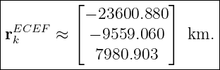
Substitution into Equations (36), (37), and (38) gives
In kilometers,
A final norm check gives
which verifies that the final transformation changed only coordinate orientation, not physical
distance from Earth.
12 Sanity checks and implementation traps
1. Keep Φk and uk distinct
The harmonic corrections are evaluated using
not 2uk. First compute δuk, then form uk = Φk + δuk.
2. Keep the three correction units distinct
The correction channels have different dimensions:
Adding a radial coefficient to an angle or vice versa is a detectable unit error.
3. Convert semicircle quantities before mixing them
Cuc,Cus,Cic,Cis are already specified in radians, but i0, Ω0,  , and IDOT are broadcast in
semicircle-based units. Convert them before using Equations (22) and (30).
, and IDOT are broadcast in
semicircle-based units. Convert them before using Equations (22) and (30).
4. Check both coordinate norms
The two identities
and
should hold to numerical precision. The first tests the polar decomposition; the second tests the
rotation into ECEF.
5. Do not apply Earth rotation twice
The node equation already includes the Earth-rate term. The final Table 20-IV coordinates are
ECEF, not ECI.
6. Zero-correction limit
If
then
This recovers the uncorrected Keplerian geometry except for the separately modeled node
evolution.
7. Equatorial limit
For
Equation (38) gives
and the x-y equations reduce to an ordinary planar rotation by Ωk.
13 Compact implementation sequence
Given the outputs of GPSORB12 and the remaining decoded ephemeris parameters:
-
1.
- Evaluate sin 2Φk and cos 2Φk once.
-
2.
- Compute δuk, δrk, and δik.
-
3.
- Form uk = Φk + δuk.
-
4.
- Form rk = A(1 − e cos Ek) + δrk.
-
5.
- Form ik = i0 + IDOT tk + δik.
-
6.
- Compute x′k = rk cos uk and y′k = rk sin uk.
-
7.
- Compute Ωk = Ω0 + (
 −
− e)tk −
 etoe.
etoe.
-
8.
- Compute xk,yk,zk from Equations (36), (37), and (38).
-
9.
- Verify
 ≈ rk.
≈ rk.
A practical implementation can reduce repeated trigonometric work by caching
14 How the equations map back to the mechanics
The second half of Table 20-IV is not an arbitrary list of coordinate recipes. Each group has a clear
origin:
| Broadcast equation | Underlying idea |
| δuk,δrk,δik | fitted twice-per-revolution departures from the
Keplerian baseline |
| uk,rk,ik | corrected orbital geometry |
| x′k,y′k | polar-to-Cartesian coordinates in the node-aligned
orbital plane |
| Ωk | node propagation relative to rotating Earth-fixed axes |
| xk,yk,zk | rigid rotation from corrected orbital-plane coordinates
into WGS 84 ECEF |
The full legacy position algorithm can now be read as one continuous chain from Newtonian orbit
parameters to an Earth-fixed satellite position:
15 Summary
Starting with the uncorrected argument of latitude from GPSORB12,
Table 20-IV forms
The corrected geometry is
The node-aligned orbital-plane coordinates are
and the Earth-fixed node longitude is
Finally,
which completes the legacy broadcast calculation of the satellite’s WGS 84 ECEF position.
The next article can continue to Table 20-IV sheet 3 and derive the satellite velocity equations
analytically by differentiating this complete position chain.
References
[1] Global Positioning Systems Directorate, IS-GPS-200N: NAVSTAR GPS Space
Segment/Navigation User Interfaces, 1 August 2022, especially Tables 20-III and 20-IV
and Section 20.3.3.4. Available from GPS.gov.
[2] GPS.gov, Interface Control Documents (ICDs) and Interface Specifications (ISs),
current public-document index, accessed September 2026.
[3] E. D. Kaplan and C. J. Hegarty, eds., Understanding GPS/GNSS: Principles and
Applications, 3rd ed., Artech House, 2017.
[4] D. A. Vallado, Fundamentals of Astrodynamics and Applications, 4th ed., Microcosm
Press, 2013.
[5] O. Montenbruck and E. Gill, Satellite Orbits: Models, Methods, and Applications,
Springer, 2000.









![[δuk] = rad.](https://images.physicslibrary.org/cache/objects/1268/make4ht/DerivingISGPS200Table20IVHarmonicCorrectionsOrbitalPlaneCoordinatesAndECEFPosition11x.png)




![[δrk] = m.](https://images.physicslibrary.org/cache/objects/1268/make4ht/DerivingISGPS200Table20IVHarmonicCorrectionsOrbitalPlaneCoordinatesAndECEFPosition16x.png)




![[δik] = rad.](https://images.physicslibrary.org/cache/objects/1268/make4ht/DerivingISGPS200Table20IVHarmonicCorrectionsOrbitalPlaneCoordinatesAndECEFPosition21x.png)














































![[δuk ] = rad, [δrk] = m, [δik] = rad.](https://images.physicslibrary.org/cache/objects/1268/make4ht/DerivingISGPS200Table20IVHarmonicCorrectionsOrbitalPlaneCoordinatesAndECEFPosition77x.png)